Chapter 3 Samples of Writing in `R bookdown`

In this chapter, you learn how to:

Reference other sections and equations
Include in-text citation that links to the bibliography
Include tables and figures not generated by R code
Include a footnote
Add tooltip descriptions for technical phrases
Include chapter examples and R code

As we expand our contributor and reviewer base, it will be helpful to know more about the conventions used in the series regarding the details of R markdown and R bookdown used in the series. This chapter summarizes these conventions.

3.1 Section Labels and Learning Objectives

The following shows how to code Section titles and refer to them.

## Section Labels {#S:SectionLabels}

With that reference, one can readily refer to Section 3.1 in your text, as follows:

With that reference, one can readily refer to 
Section \@ref(S:SectionLabels) in your text, as follows:

The following shows how to code learning objectives:

***
In this chapter, you learn how to:
  
- Reference other sections and equations
- Include in-text citation that links to the bibliography
- Include tables and figures
- Include a footnote

***

3.2 Equation References

Here is an example of a latex equation produced in R markdown, with reference number.

\[\begin{equation} x + y = 1 \tag{3.1} \end{equation}\]

You can produce that equation using the following code.

\begin{equation}
  x + y = 1  
(\#eq:ExampleEquation)
\end{equation}

With this, equation (3.1) can be referred to using the following code:

With this, equation \@ref(eq:ExampleEquation) can be 
referred to using the following code:

3.3 In-text Citations

Here is an example of an in-text citation made possible by R bookdown (Xie 2015). This links to the bibliography where the full referece is displayed. As a convention we use the APA style citation.

Here is an example of an in-text citation made possible by 
`R bookdown` [@xie2015]. This links to the bibliography 
where the full reference is displayed. 
As a convention we use the *APA* style citation.

3.4 Including Tables

We want to be able to include Latex tables (for mathematical type), as well as data-drive tables produced by R. In order to do that, we use html syntax in order to reference tables. This means that we have to number the tables by hand. Although a bit painful, it does gives us the flexibility needed.

3.4.1 Latex Generated Table

Start with a Latex generated table.

Table 2.1. An Example of Including Tables using Latex in an R markdown Document

\[ \begin{matrix} \begin{array}{c|c} \hline \text{Policyholder} & \text{Number of claims} \\\hline \textbf{X} & 1 \\\hline \textbf{Y} & 2 \\\hline \end{array} \end{matrix} \]

R markdown does not have a convention for referencing non- R generated tables. For now, we reference them manually as in refer to Table 2.1. We do this by manually inserting an html anchor tag.

The following code produces this table.

<a id=tab:2.1></a> 

[Table 2.1]: \#tab:2.1

Table 2.1. **An Example of Including Tables using Latex in an `R markdown` Document**

$$
\begin{matrix}
    \begin{array}{c|c} \hline
    \text{Policyholder} & \text{Number of claims} \\\hline
    \textbf{X} & 1 \\\hline
    \textbf{Y} & 2 \\\hline
    \end{array}
\end{matrix}
$$

For reference, then use

`R markdown` does not have a convention for referencing 
non-R generated tables. For now, we reference them manually 
as in refer to [Table 2.1].

3.4.2 Table Generated by `R`

Now we give a data-driven table generated by R in Table 2.2.

Table 2.2. An Example of Including Tables using R

Minimum	First Quartile	Median	Mean	Third Quartile	Maximum
167	2226	4951	56332	11900	12922218

Here is the code to produce this table.


<a id=tab:2.2></a> 

[Table 2.2]: \#tab:2.2

Table 2.2. **An Example of Including Tables using `R` **

```{r message = FALSE, 
   warning = FALSE, eval = FALSE, echo = TRUE}
Insample <- read.csv("Insample.csv", header=T,  
              na.strings=c("."), stringsAsFactors=FALSE)
Insample2010 <- subset(Insample, Year==2010)
InsamplePos2010 <- subset(Insample2010, yAvg>0)
summaryOutput <- t(as.matrix(summary(InsamplePos2010$yAvg)))
colnames(summaryOutput) <- c("Minimum","First Quartile", 
                             "Median", "Mean", "Third Quartile", "Maximum")
kable_styling(knitr::kable(summaryOutput,digits=0, 
                    align = "rrrrrr"), latex_options="scale_down")
```

3.5 Including Figures

For figures, we can use the same reference/label system for figures produced by R and those external to R. This makes things easier than with tables.

3.5.1 Figures Generated by `R`

Most figures are generated using R. Here is an example.

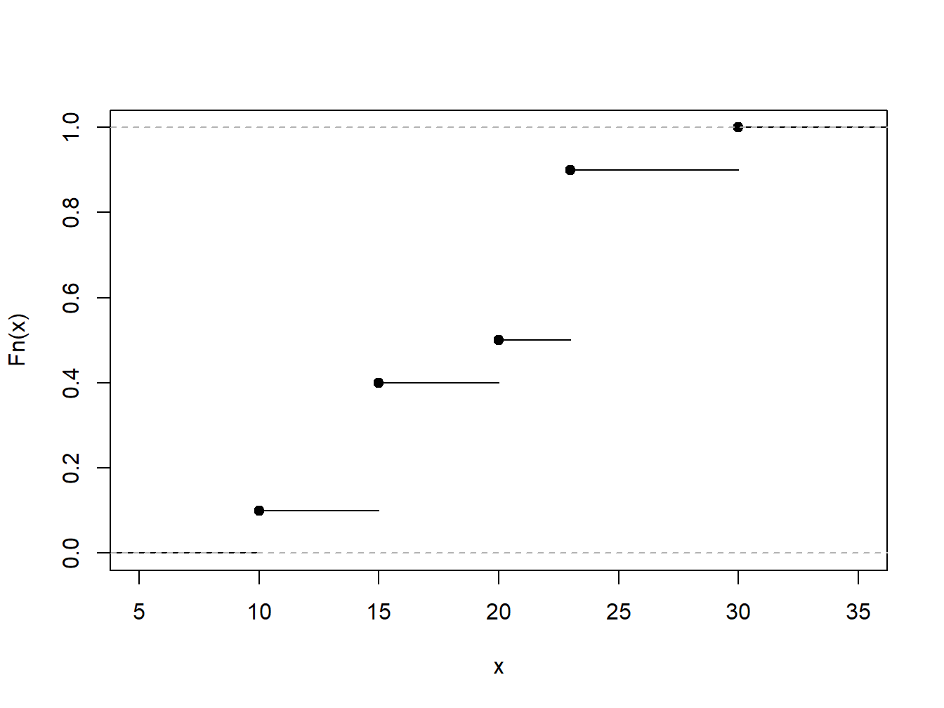
Figure 3.1: Empirical Distribution Function of a Toy Example

that we refer to as Figure 3.1. Here is the code for producing the figure:


(ref:  EDFToy) **Empirical Distribution Function of a Toy Example**

{r EDFToy, echo = FALSE, 
     fig.cap='(ref: EDFToy)', out.width = '60%', fig.asp = 0.75, fig.align = 'center'}
xExample <- c(10,rep(15,3),20,rep(23,4),30)
PercentilesxExample <- ecdf(xExample)
plot(PercentilesxExample, main = "", xlab = "x")
```

Here is is the code for referencing the Figure 3.1:

Here is is the code for referencing the Figure \@ref(fig:EDFToy):

3.5.2 Figures Not Generated by `R`

For figures, we store the figures as png or jpeg files in a separate folder called “Figures”. Then we use R code to call those figures for display so that we can reference them.

Here is such a figure:

Figure 3.2: An Example of Including Figures in an R Markdown Document

And here is the code that generates the figure:


(ref:  ExampleFigure) **An Example of Including Figures in an R Markdown Document**
    
```{r ExampleFigure, fig.cap='(ref: ExampleFigure)', 
      out.width = '5%', fig.align = 'center', echo = FALSE}
knitr::include_graphics("Figures/RStudio-Ball.png")
```

Here is is the code for referencing the Figure 3.2:

Here is is the code for referencing the Figure \@ref(fig:ExampleFigure):

3.6 Including Footnotes

Try to minimize the use of footnotes. But, if you need them, here is how you can include a footnote.²

Here is how you can include a footnote [^1].
    
[^1]: the footnote displays at the end of the chapter

3.7 Defining Glossary Terms

Use the Gloss(term) function to include a tooltip for technical phrases. Gloss(term) looks up the definition in GlossFct.csv. Accordingly, you can add new glossary terms for your chapter in the csv file.

Here is how you add a tooltip:

We can use the same Gloss(term) function to include tooltips for acronyms (e.g. iid) as listed in Section 4.2.

3.7.1 Glossary Conventions

Include tooltip for a term only once in a chapter.
Include tooltip when the term is defined. (e.g. “Frequency is …”)
If term is not explicitly defined, include tooltip at the term’s first occurence in the chapter.
Only include tooltip in the Chapter Preview or in examples if the term is not defined elsewhere in the chapter.

3.7.2 Glossary Terms with Multiple Definitions

A term may carry multiple definitions across different sections. In this case, use Gloss(term, section):

3.8 Including Chapter Examples and R Code

As described in Section 2, chapter examples and R code allow readers to interact with the online version of the book.

Here is how to add a chapter example:

Show Example Solution

"single backtick"r HideExample('5.2.1', 'Show Example Solution')"single backtick"

**insert solution here**

</div>

Similarly, you can add statistical code:

R Code for Pearson Correlation Statistic

"single backtick"r HideRCode('pearson.1','R Code for Pearson Correlation Statistic')"single backtick"

# insert R codeblock here with {r echo=SHOW_PDF}

</div>

and also proof theory:

Show Technical Details

"single backtick"r HideProofTheory('LTV.1',"Show Technical Details")"single backtick"

**Solution**

$$E = m c^2$$

</div>

HideExample, HideRCode, and HideProofTheory are R functions that can hide these interactive features in the online html version. In the offline (pdf) version of the book, these are suppressed. All you need to do is change eval = TRUE in the file PdfOutput.Rmd.

3.9 Useful Links

Naturally, you will want to learn more about coding in R markdown, R bookdown and so forth. The following provide some useful links for taking the next step.

For an R markdown guide refer https://rmarkdown.rstudio.com/authoring_pandoc_markdown.html.
For a R bookdown guide, see https://bookdown.org/yihui/bookdown/.
For best practices in coding R, we suggest http://r-pkgs.had.co.nz/style.html.
See also our online actuarial text resources at https://sites.google.com/a/wisc.edu/loss-data-analytics/online-actuarial-text-resources.

the footnote displays at the end of the chapter↩

Chapter 3 Samples of Writing in R bookdown