Chapter 12 Experience Rating using Bonus-Malus
This chapter is being written and is not yet complete nor edited. It is here to give you a flavor of what will be in the final version.
12.1 Introduction
Bonus-malus system, which is used interchangeably as “no-fault discount”, “merit rating”, “experience rating” or “no-claim discount” in different countries, is based on penalizing insureds who are responsible for one or more claims by a premium surcharge, and awarding insureds with a premium discount if they do not have any claims. Insurers use bonus-malus systems for two main purposes; to encourage drivers to drive more carefully in a year without any claims, and to ensure insureds to pay premiums proportional to their risks based on their claims experience.
No Claim Discount (NCD) system is an experience rating system commonly used in motor insurance. It represents an attempt to categorize insureds into homogeneous groups who pay premiums based on their claims experience. Depending on the rules in the scheme, new policyholders may be required to pay full premium initially, and obtain discounts in the future years as a results of claim-free years. An NCD system rewards policyholders for not making any claims during a year, or in other words, it grants a bonus to a careful driver. This bonus principle may affect policy holders’ decisions whether to claim or not to claim, especially when involving accidents with slight damages, which is known as ‘hunger for bonus’ phenomenon. The option of ‘hunger for bonus’ under an NCD system may reduce insurers’ claim costs, and may be able to offset the expected decrease in premium income.
12.2 NCD System in Several Countries
12.2.1 NCD System in Malaysia
Before the liberalization of Motor Tariff on 1st July 2017, the rating of motor insurance in Malaysia was governed by Motor Tariff. Under the tariff, the rate charged should not be lower than the rates specified under the classes of risks, to ensure that the price competition among insurers will not go below the country’s economic level. The basic rating factors considered were scope of insurance, cubic capacity of vehicle and estimated value of vehicle (or sum insured, whichever is lower). Under the Motor Tariff, the final premium to be paid is adjusted by the policyholder’s claim experience, or equivalently, his NCD entitlement.
Effective on 1st July 2017, the premium rates for motor insurance are liberalized, or de-tariffed. The pricing of premium is now determined by individual insurers and takaful operators, and the consumers are able to enjoy a wider choice of motor insurance products at competitive prices. Since tariff liberalization encourages innovation and competition among insurers and takaful operators, the premiums are based on broader risk factors other than the two rating factors specified in the Motor Tariff, i.e. sum insured and cubic capacity of vehicle. Other rating factors may be defined in the risk profile of an insured, such as age of vehicle, age of driver, safety and security features of vehicle, geographical location of vehicle and traffic offences of driver. As different insurers and takaful operators have different ways of defining the risk profile of an insured, the price of a policy may differ from one insurer to another. However, the NCD structure from the Motor Tariff remains ‘unchanged’ and continue to exist, and is ‘transferable’ from one insurer, or from one takaful operator, to another.
The discounts in the Malaysian NCD system are divided into six classes, starting from the initial class of 0% discount, followed by classes of 25%, 30%, 38.3%, 45% and 55% discounts. Table 1 provides the classes of NCD system in Malaysia. A claim-free year indicates that a policyholder is entitled to move one-step forward to the next discount class, such as from a 0% discount to a 25% discount in the renewal year. If a policyholder is already at the highest class, which is at a 55% discount, a claim-free year indicates that the policyholder remains in the same class. On the other hand, if one or more claims are made within the year, the NCD will be forfeited and the policyholder has to start at 0% discount in the renewal year. In other words, the policyholder has to pay a full premium for the next year’s renewal premium, regardless of his current class of NCD.
For an illustration purpose, Figure 12.1 shows the transition diagram for the NCD classes under the Malaysian Motor Tariff. The transition starts at class 0, and increase one by one if an insured has a no-claim year. If an insured has one or more claims within the year, the current class automatically returns to class 0.
\[ \begin{matrix} \text{Table 1: Classes of NCD (Malaysia)}\\ \begin{array}{*{20}c} \hline \text{Classes (claim-free years)} & \text{Discounts}\\ \hline\\ {0} & {0}\\ {1} & {25}\\ {2} & {30}\\ {3} & {38.33}\\ {4} & {45}\\ {5\text{ and above}} & {55}\\\\ \hline \end{array} \end{matrix} \]
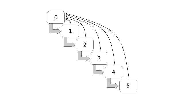
Figure 12.1: Transition diagram for NCD classes (Malaysia)
12.2.2 NCD System in Other Countries
The NCD system in Brazil are subdivided into seven classes, with the following premium levels (Lemaire 1998): 100, 90, 85, 80, 75, 70, and 65. These premium levels are also equivalent to the following discount classes: 0%, 10%, 15%, 20%, 25%, 30% and 45%. New policyholders have to start at 0% discount, or at level 100, and a claim-free year indicates that a policyholder can move forward at a one-class discount. If one or more claims incurred within the year, the policyholder has to move backward, also at a one-class discount. Table 2 and Figure 12.2 respectively show the classes and the transition diagram for the NCD system in Brazil.
\[ \begin{matrix} \text{Table 2: Classes of NCD (Brazil)}\\ \begin{array}{*{20}c} \hline \text{Classes (claim-free years)} & \text{Discounts}\\ \hline\\ {0} & {0}\\ {1} & {10}\\ {2} & {15}\\ {3} & {20}\\ {4} & {25}\\ {5} & {30}\\ {6\text{ and above}} & {45}\\\\ \hline \end{array} \end{matrix} \]
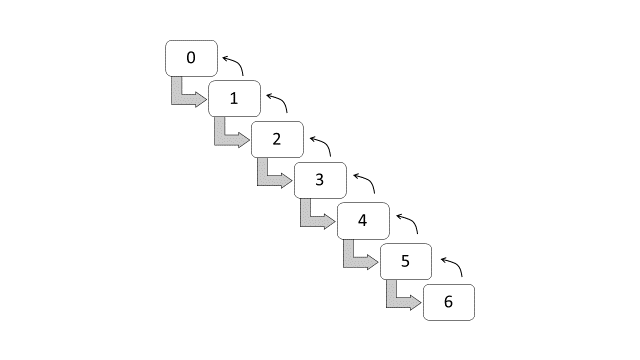
Figure 12.2: Transition diagram for NCD classes (Brazil)
The NCD system in Switzerland, which is implemented in 1990, are subdivided into twenty-two classes, with the following premium levels: 270, 250, 230, 215, 200, 185, 170, 155, 140, 130, 120, 110, 100, 90, 80, 75, 70, 65, 60, 55, 50 and 45 (Lemaire and Zi 1994). These levels are also equivalent to the following loadings: 170%, 150%, 130%, 115%, 100%, 85%, 70%, 55%, 40%, 30%, 20%, and 10%, and the following discounts: 0%, 10%, 20%, 25%, 30%, 35%, 40%, 45%, 50% and 55%. New policyholders have to start at 170% loading, or at 270 premium level, and a claim-free year indicates that a policyholder can move one-class forward. If one or more claims incurred within the year, the policyholder has to move four-classes backwards. Table 3 and Figure 12.3 respectively show the classes and the transition diagram for the NCD system in Switzerland.
\[ \begin{matrix} \text{Table 3: Classes of NCD (Switzerland)}\\ \begin{array}{*{20}c} \hline \text{Classes} & \text{Loadings} & \text{Classes} & \text{Discounts}\\ \text{(claim-free years)} & & \text{(claim-free years)} & \\ \hline\\ {0} & {170} & {12} & {0}\\ {1} & {150} & {13} & {10}\\ {2} & {130} & {14} & {20}\\ {3} & {115} & {15} & {25}\\ {4} & {100} & {16} & {30}\\ {5} & {85} & {17} & {35}\\ {6} & {70} & {18} & {40}\\ {7} & {55} & {19} & {45}\\ {8} & {40} & {20} & {50}\\ {9} & {30} & {21 \text{ and above}} & {55}\\ {10} & {20} && \\ {11} & {10} && \\\\ \hline \end{array} \end{matrix} \]
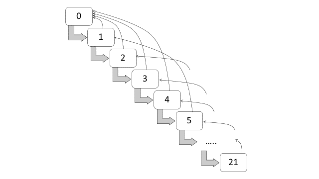
Figure 12.3: Transition diagram for NCD classes (Switzerland)
12.3 BMS and Markov Chain Model
A BMS, or an NCD system, can be represented by a discrete time parameter Markov chain. Under this model, the state space consists of classes of bonus-malus, and the state (or class) is assumed to shift randomly from year to year. Therefore, it is important to know a brief description on two elements; a stochastic process that has a Markov property, and a discrete time Markov chain.
Definition: A stochastic process has a Markov property if the probability distribution of future states, conditional on both past and present states, depends only upon the present state and not on the sequence of events that preceded it.
Definition: A discrete time Markov chain is a stochastic process that can be parameterized by empirically estimating the transition probabilities between discrete states.
12.3.1 Transition Probability
The randomness of the transition of the NCD classes is governed by the transition probability in a given year. The definition of a transition probability is provided here to understand the use of the probability for representing the transition of the NCD classes.
Definition: The transition probability from state \(i\) (at time \(n\)) to state \(j\) (at time \(n + 1\)) is called a one-step transition probability, and is denoted by \(p_{ij} = Pr (X_{n + 1} = j|X_n = i)\), \(i = 1,2,...,k\), \(j = 1,2,...,k\).
The transition probabilities can be represented by a \(k \times k\) matrix. Assuming a homogeneous Markov process, a k-state Markov chain can be represented by a matrix of transition probabilities \({\bf P}\):
\[ {\bf P} = \left[ {\begin{array}{*{20}c} p_{11} & p_{12} & \ldots & & & p_{1k} \\ p_{21} & p_{22} & \ldots & & & p_{2k} \\ \vdots & \ddots & & & & \vdots \\ & & & & & \\ & & & & & \\ p_{k1} & p_{k2} & \cdots & & & p_{kk} \end{array} } \right]. \]
Each row of the transition matrix represents the transition of flowing out of state, whereas each column represents the transition of flowing into the state. The cumulative transitions of flowing out of state must equal 1, or each row of the matrix must sum to 1, i.e. \(\sum\limits_j p_{ij} = 1\). All probabilities must also be non-negative (since they are probabilities), i.e. \(p_{ij} \ge 0\).
Consider the Malaysian NCD system. Under this system, let the random variable \(X_t\) denotes the class of NCD at time \(t\) and takes the values in a state space \(\bf{S}\), where \({\bf S} = \{0,1,...,5\}\). Therefore, the probability of a no-claim year is equal to the probability of transition from state \(i\) to state \(j\), which is \(p_{ij}\), \(i = 0,1,2,...,5\), \(j = 0,1,2,...,5\). If an insured has one or more claims within the year, the probability of transitioning back to state 0 is represented by \(p_{i0}\), which is also equivalent to \(1 - {p_{ij}}.\) Therefore, there are only two transition probabilities in each row; the probability of advancing to the next state, \(p_{ij},\) and the probability of returning back to state zero, \(p_{i0} = 1 - p_{ij}\).
In terms of transition probabilities, the Malaysian NCD system can be represented by the following \((6 \times 6)\) transition matrix:
\[ {\bf P} = \left[ {\begin{array}{*{20}c} p_{00}&p_{01}&0&0&0&0\\ p_{10}&0&p_{12}&0&0&0\\ p_{20}&0&0&p_{23}&0&0\\ p_{30}&0&0&0&p_{34}&0\\ p_{40}&0&0&0&0&p_{45}\\ p_{50}&0&0&0&0&p_{55} \end{array} }\right] = \left[ {\begin{array}{*{20}c} {1 - p_{01}}&p_{01}&0&0&0&0\\ {1 - p_{12}}&0&p_{12}&0&0&0\\ {1 - p_{23}}&0&0&p_{23}&0&0\\ {1 - p_{34}}&0&0&0&p_{34}&0\\ {1 - p_{45}}&0&0&0&0&p_{45}\\ {1 - p_{55}}&0&0&0&0&p_{55} \end{array} }\right] \]
Example 1
Provide the transition matrix for the NCD system in Brazil.
Solution
Based on the NCD classes and the transition diagram shown respectively in Table 2 and Figure 12.2, the probability of a no-claim year is equal to the probability of moving one-class forward, whereas the probability of having one or more claims within the year is equal to the probability of moving one-class backward. Therefore, each row can contain two or more transition probabilities; one probability for advancing to the next state, and one or more probabilities for moving one-class backwards. The transition matrix is:
\[ {\bf P} = \left[ {\begin{array}{*{20}{c}} {1 - p_{01}}&p_{01}&0&0&0&0&0\\ {1 - p_{12}}&0&p_{12}&0&0&0&0\\ {1 - \sum\limits_j p_{2j}}&p_{21}&0&p_{23}&0&0&0\\ {1 - \sum\limits_j p_{3j}}&p_{31}&p_{32}&0&p_{34}&0&0\\\ {1 - \sum\limits_j p_{4j}}&p_{41}&p_{42}&p_{43}&0&p_{45}&0\\ {1 - \sum\limits_j p_{5j}}&p_{51}&p_{52}&p_{53}&p_{54}&0&p_{56}\\ {1 - \sum\limits_j p_{6j}}&p_{61}&p_{62}&p_{63}&p_{64}&p_{65}&p_{66} \end{array} } \right] \]
Example 2
Provide the transition matrix for the NCD system in Switzerland.
Solution
From Table 3 and Figure 12.3, the probability of a no-claim year is equal to the probability of moving one-class forward, whereas the probability of having one or more claims within the year is equal to the probability of moving four-classes backward. The transition matrix is:
\[ \begin{matrix} \left| {\begin{array}{*{12}{c}} 1 - {p_{01}} & p_{01} & 0 & 0 & 0 & 0 & 0 & 0 & 0 & 0 & 0 & \cdots\\ 1 - {p_{12}} & 0 & p_{12} & 0 & 0 & 0 & 0 & 0 & 0 & 0 & 0 & \cdots\\ 1 - {p_{23}} & 0 & 0 & p_{23} & 0 & 0 & 0 & 0 & 0 & 0 & 0 & \cdots\\ 1 - {p_{34}} & 0 & 0 & 0 & p_{34} & 0 & 0 & 0 & 0 & 0 & 0 & \cdots\\ 1 - {p_{45}} & 0 & 0 & 0 & 0 & p_{45} & 0 & 0 & 0 & 0 & 0 & \cdots\\ 1 - \sum\limits_j {p_{5j}} & p_{51} & 0 & 0 & 0 & 0 & p_{56} & 0 & 0 & 0 & 0 & \cdots\\ 1 - \sum\limits_j {p_{6j}} & 0 & p_{62} & 0 & 0 & 0 & 0 & p_{67} & 0 & 0 & 0 & \cdots\\ 1 - \sum\limits_j {p_{7j}} & 0 & 0 & p_{73} & 0 & 0 & 0 & 0 & p_{78} & 0 & 0 & \cdots\\ \vdots & \vdots & \vdots & \vdots & \vdots & \vdots & \vdots & \vdots & \vdots & \vdots & \vdots & \ddots\\ 1 - \sum\limits_j {p_{19,j}} & 0 & 0 & p_{19,3} & 0 & 0 & 0 & p_{19,7} & 0 & 0 & 0 & \cdots\\ 1 - \sum\limits_j {p_{20,j}} & 0 & 0 & 0 & p_{20,4} & 0 & 0 & 0 & p_{20,8} & 0 & 0 & \cdots\\ 1 - \sum\limits_j {p_{21,j}} & p_{21,1} & 0 & 0 & 0 & p_{21,5} & 0 & 0 & 0 & p_{21,9} & 0 & \cdots \end{array}} \right| \end{matrix} \]
12.4 BMS and Stationary Distribution
12.4.1 Stationary Distribution
It is important to note that the transition matrix represents the transition probabilities of the NCD classes in one year. If we are interested in the distribution of the transition in the long run (which may take several years), the stationary probability can be used.
Several definitions and properties are provided here to understand the use of a Markov chain model for representing the stationary distribution of the NCD transitions. However, students are encouraged to refer to textbooks on Markov Chain and stochastic processes available in the literature for a more comprehensive knowledge on the related subjects.
Definition: A Markov chain is said to be irreducible if it is possible to move to any state from any other state.
Definition: A state \(i\) has period \(k\) if any return to state \(i\) must occur in multiples of \(k\) time steps. If \(k = 1\), then the state is said to be aperiodic.
Definition: A state \(i\) is said to be transient if, given that we start in state \(i\), there is a non-zero probability that we will never return to \(i\). State \(i\) is recurrent (or persistent) if it is not transient. A state \(i\) is positive recurrent if the mean recurrent time (or expected return time) is finite.
Definition: A state \(i\) is said to be ergodic if it is aperiodic and positive recurrent. In other words, a state \(i\) is ergodic if it is recurrent, has a period of one (aperiodic), and has finite mean recurrence time. If all states in an irreducible Markov chain are ergodic, then the chain is said to be ergodic.
Definition: Let \(p_{ij}^{(n)} = \Pr ({X_n} = j\|{X_0} = i)\) be the probability of transition from state \(i\) to state \(j\) in \(n\) time steps. The n-step transition probabilities for a stationary Markov chain satisfy the Chapman–Kolmogorov equation:
\[p_{ij}^{(n)} = \sum\limits_r {p_{ir}^{(k)}p_{rj}^{(n - k)}}\]
for any \(k\), where \(0 < k < n\).
Definition: If a Markov chain is stationary, then the vector \({\bf{\pi }}\) is called a stationary distribution (or invariant measure) if it satisfies:
\[0 \le {\pi _j} \le 1\]
\[\sum\limits_j {{\pi _j}} = 1,\]
\[{\pi_j} = \sum\limits_i {\pi_i}p_{ij}\].
In terms of vectors and matrices, a stationary distribution \({\bf{\pi }}\) is a row vector, whose entries are non-negative and sum to one, that is unchanged by the operation:
\({\bf{\pi P}} = {\bf{\pi }}\).
If a Markov chain is stationary, then the transition matrix \({\bf{P}}\) is the same after each step, so that the \(k\)-step transition probability can be computed as the \(k\)-th power of the transition matrix, \({{\bf{P}}^k}.\)
From the definitions and properties above, a BMS forms a regular Markov chain if all of its states (NCD classes) are ergodic, and the chain is not cyclic (or irreversible). The row vector, \({\bf{\pi }}\), which is also the left eigenvector of the transition matrix, is a stationary distribution defined by \(0 \le {\pi _j} \le 1\) and \(\sum\limits_j {{\pi_j}} = 1\).
Example 3
Find the stationary distribution for the NCD system in Malaysia assuming that the probability of a no-claim year for all NCD classes are \({p_0}\).
Solution
The transition matrix can be re-written as:
The stationary distribution can be calculated using \({\pi _j} = \sum\limits_i {\pi _i}p_{ij}\). The solutions are:
\[ \begin{array}{l} {\pi _0} = \sum\limits_i {\pi_i}p_{i0} = (1 - {p_0})\sum\limits_i {{\pi _i}} = 1 - {p_0}\\\\ {\pi _1} = \sum\limits_i {\pi _i}p_{i1} = {\pi_0}{p_{01}} = (1 - {p_0}){p_0}\\\\ {\pi _2} = \sum\limits_i {\pi _i}p_{i2} = {\pi _1}{p_{12}} = (1 - {p_0}){p_0}^2\\\\ {\pi _3} = \sum\limits_i {\pi _i}p_{i3} = {\pi _2}{p_{23}} = (1 - {p_0}){p_0}^3\\\\ {\pi _4} = \sum\limits_i {\pi _i}p_{i4} = {\pi _3}{p_{34}} = (1 - {p_0}){p_0}^4\\\\ {\pi _5} = \sum\limits_i {\pi _i}p_{i5} = {\pi _4}{p_{45}} + {\pi _5}{p_{55}} = (1 - {p_0}){p_0}^5 + {\pi _5}{p_0}\\\\ \therefore {\pi _5} = \frac{(1 - {p_0}){p_0}^5}{{(1 - {p_0})}} = {p_0}^5 \end{array} \]
The stationary distribution (or steady state condition) shown in Example 3 represents the asymptotic distribution of the NCD system, or the distribution in the long run. As an example, assuming that the probability of a no-claim year is \(p_0 = 0.90,\) the stationary probabilities are:
\[ \begin{array}{l} {\pi _0} = 1 - {p_0} = 0.1000\\\\ {\pi _1} = (1 - {p_0}){p_0} = 0.0900\\\\ {\pi _2} = (1 - {p_0}){p_0}^2 = 0.0810\\\\ {\pi _3} = (1 - {p_0}){p_0}^3 = 0.0729\\\\ {\pi _4} = (1 - {p_0}){p_0}^4 = 0.0656\\\\ {\pi _5} = {p_0}^5 = 0.5905 \end{array} \]
In other words, \({\pi_0} = 0.10\) indicates that 10% of insureds will eventually belong to class 0 (or zero claim-free years), \({\pi _1} = 0.09\) indicates that 9% of insureds will eventually belong to class 1 (or one claim-free year), and so forth, until \({\pi _5} = 0.59\), which indicates that 59% of insureds will eventually belong to class 5 (or five successive claim-free years).
12.4.2 R Program for Stationary Distribution
We can use the left eigenvector of a transition matrix to calculate the stationary distribution. The following R program can be used to calculate the left eigenvector:
#create transition matrix
entries=c(0.1,0.9,0,0,0,0,
+ 0.1,0,0.9,0,0,0,
+ 0.1,0,0,0.9,0,0,
+ 0.1,0,0,0,0.9,0,
+ 0.1,0,0,0,0,0.9,
+ 0.1,0,0,0,0,0.9)
TP=matrix(entries,nrow=6,byrow=TRUE)
TP
## [,1] [,2] [,3] [,4] [,5] [,6]
## [1,] 0.1 0.9 0.0 0.0 0.0 0.0
## [2,] 0.1 0.0 0.9 0.0 0.0 0.0
## [3,] 0.1 0.0 0.0 0.9 0.0 0.0
## [4,] 0.1 0.0 0.0 0.0 0.9 0.0
## [5,] 0.1 0.0 0.0 0.0 0.0 0.9
## [6,] 0.1 0.0 0.0 0.0 0.0 0.9#calculate left eigenvector
#hint -- left eigenvector is the same as right eigenvector of transpose of transition matrix
eigen(t(TP))## eigen() decomposition
## $values
## [1] 1.0000000000+0.0000000000i -0.0004880382+0.0003546725i
## [3] -0.0004880382-0.0003546725i 0.0001865015+0.0005736028i
## [5] 0.0001865015-0.0005736028i 0.0006030733+0.0000000000i
##
## $vectors
## [,1] [,2]
## [1,] 0.1615936+0i 0.00000000000011546+0.0000000000000838874i
## [2,] 0.1454342+0i -0.00000000006591101-0.0000000002025976972i
## [3,] 0.1308908+0i -0.00000009813867774+0.0000003022936262135i
## [4,] 0.1178017+0i 0.00038354290934278-0.0002787325538732070i
## [5,] 0.1060216+0i -0.70729837066103896+0.0000000000000000000i
## [6,] 0.9541940+0i 0.70691492595616912+0.0002784304627608034i
## [,3]
## [1,] 0.00000000000011546-0.0000000000000838874i
## [2,] -0.00000000006591101+0.0000000002025976972i
## [3,] -0.00000009813867774-0.0000003022936262135i
## [4,] 0.00038354290934278+0.0002787325538732070i
## [5,] -0.70729837066103896+0.0000000000000000000i
## [6,] 0.70691492595616912-0.0002784304627608034i
## [,4]
## [1,] -0.0000000000000440003+0.0000000000001357099i
## [2,] 0.0000000001723292683+0.0000000001248792837i
## [3,] 0.0000002567150759536-0.0000001869214542640i
## [4,] -0.0001468014877601952-0.0004505247500856750i
## [5,] -0.7070333538878578183+0.0004507115465249567i
## [6,] 0.7071798984882565753+0.0000000000000000000i
## [,5] [,6]
## [1,] -0.0000000000000440003-0.0000000000001357099i 0.0000000000001426323+0i
## [2,] 0.0000000001723292683-0.0000000001248792837i 0.0000000002126778891+0i
## [3,] 0.0000002567150759536+0.0000001869214542640i 0.0000003173909504803+0i
## [4,] -0.0001468014877601952+0.0004505247500856750i 0.0004736602551468477+0i
## [5,] -0.7070333538878578183-0.0004507115465249567i 0.7068696732221422252+0i
## [6,] 0.7071798984882565753+0.0000000000000000000i -0.7073436510810596767+0i#divide entry of first column by sum of elements, so that entries sum to 1
#provide answers in 4 decimal places
round(eigen(t(TP))$vectors[,1]/sum(eigen(t(TP))$vectors[,1]),4)## [1] 0.1000+0i 0.0900+0i 0.0810+0i 0.0729+0i 0.0656+0i 0.5905+0iExample 4
Find the stationary distribution for the NCD system in Brazil assuming that the number of successive years of claims is Poisson distributed with parameter \(\lambda = 0.10\).
Solution
Under the Poisson distribution, the probability of \(k\) successive years of claims is \(p_k = \frac{e^{ - 0.1}{(0.1)}^k}{{k!}},{\rm{ }}k = 0,1,2,.....\)
The transition matrix is:
\[ {\small {\bf{P}} = \left[ {\begin{array}{*{20}{c}} {1 - {p_0}}&{{p_0}}&0&0&0&0&0\\\\ {1 - {p_0}}&0&{{p_0}}&0&0&0&0\\\\ {1 -\sum\limits_i {{p_i}} }&{{p_1}}&0&{{p_0}}&0&0&0\\\\ {1 -\sum\limits_i {{p_i}} }&{{p_2}}&{{p_1}}&0&{{p_0}}&0&0\\\\ {1 - \sum\limits_i {{p_i}}}&{{p_3}}&{{p_2}}&{{p_1}}&0&{{p_0}}&0\\\\ {1 - \sum\limits_i{{p_i}} }&{{p_4}}&{{p_3}}&{{p_2}}&{{p_1}}&0&{{p_0}}\\\\ {1 - \sum\limits_i {{p_i}}}&{{p_5}}&{{p_4}}&{{p_3}}&{{p_2}}&{{p_1}}&{{p_0}} \end{array}} \right] = \left[ {\begin{array}{*{20}{c}} {0.0952}&{0.9048}&0&0&0&0&0\\\\ {0.0952}&0&{0.9048}&0&0&0&0\\\\ {0.0047}&{0.0905}&0&{0.9048}&0&0&0\\\\ {0.0002}&{0.0045}&{0.0905}&0&{0.9048}&0&0\\\\ {0.0000}&{0.0002}&{0.0045}&{0.0905}&0&{0.9048}&0\\\\ {0.0000}&{0.0000}&{0.0002}&{0.0045}&{0.0905}&0&{0.9048}\\\\ {0.0000}&{0.0000}&{0.0000}&{0.0002}&{0.0045}&{0.0905}&{0.9048} \end{array}}\right]} \]
Using R program, the stationary probabilities are:
\[ \left[ {\begin{array}{*{20}{c}} {{\pi _0}}\\\\ {{\pi_1}}\\\\ {{\pi _2}}\\\\ {{\pi _3}}\\\\ {{\pi _4}}\\\\ {{\pi_5}}\\\\ {{\pi _6}} \end{array}} \right] = \left[ {\begin{array}{*{20}{c}} {0.0000}\\\\ {0.0000}\\\\ {0.0003}\\\\ {0.0022}\\\\ {0.0145}\\\\ {0.0936}\\\\ {0.8894} \end{array}} \right] \]
The probabilities indicate that 89% of insureds will eventually belong to class 6 (six successive claim-free years), 9% of insureds will eventually belong to class 5 (five successive claim-free years), and 1.5% of insureds will eventually belong to class 4 (four successive claim-free years). Other classes, after combined, have less than 1% of insureds.
Example 5
Using the results from Example 4, find the final premium under the steady state condition assuming that the premium prior to implementing the NCD is \(m.\)
Solution
Using the stationary probabilities from Example 4, the stationary final premium is:
\[ \begin{array}{l} = \sum\limits_j \text{(premium)} \times \text{(proportion in class } j \text{ in the long run)} \times \text{(1 - NCD in class } j)\\\\ = m[{\pi _0}(1) + {\pi _1}(1 - 0.9) + {\pi _2}(1 - 0.15) + \ldots + {\pi _6}(1 - 0.35)]\\\\ = m[0 + 0 + (0.0003)(0.85) + \ldots + (0.8894)(0.65)]\\\\ = 0.6565m \end{array} \]
The results indicate that the final premium reduce from m to 0.6565m in the long run (under steady state condition or stationary condition) if the NCD is considered.
12.4.4 R Program for Premium Evolution
The following R program can be used to find the premium in the n-th year and the premiums in 20 years under the NCD system in Malaysia (to find the solution in Example 6).
#create transition matrix
entries=c(0.0952,0.9048,0,0,0,0,
+ 0.0952,0,0.9048,0,0,0,
+ 0.0952,0,0,0.9048,0,0,
+ 0.0952,0,0,0,0.9048,0,
+ 0.0952,0,0,0,0,0.9048,
+ 0.0952,0,0,0,0,0.9048)
TP=matrix(entries,nrow=6,byrow=TRUE)
TP
## [,1] [,2] [,3] [,4] [,5] [,6]
## [1,] 0.0952 0.9048 0.0000 0.0000 0.0000 0.0000
## [2,] 0.0952 0.0000 0.9048 0.0000 0.0000 0.0000
## [3,] 0.0952 0.0000 0.0000 0.9048 0.0000 0.0000
## [4,] 0.0952 0.0000 0.0000 0.0000 0.9048 0.0000
## [5,] 0.0952 0.0000 0.0000 0.0000 0.0000 0.9048
## [6,] 0.0952 0.0000 0.0000 0.0000 0.0000 0.9048#create function for nth power of square matrix
powA = function(n) {
if (n==1) return (TP)
if (n==2) return (TP%*%TP)
if (n>2) return ( TP%*%powA(n-1)) }
#example for n=3
powA(3)## [,1] [,2] [,3] [,4] [,5] [,6]
## [1,] 0.0952 0.08613696 0.07793672 0.7407263 0.0000000 0.0000000
## [2,] 0.0952 0.08613696 0.07793672 0.0000000 0.7407263 0.0000000
## [3,] 0.0952 0.08613696 0.07793672 0.0000000 0.0000000 0.7407263
## [4,] 0.0952 0.08613696 0.07793672 0.0000000 0.0000000 0.7407263
## [5,] 0.0952 0.08613696 0.07793672 0.0000000 0.0000000 0.7407263
## [6,] 0.0952 0.08613696 0.07793672 0.0000000 0.0000000 0.7407263#define NCD percentage
NCD=c(1,.75,.7,.6167,.55,.45)
#create function for premium in nth year
p=numeric(0)
prem=function(n){
for (j in 1:length(NCD))
p[j]=mean(powA(n)[,j])
+ 100*sum(p*NCD)}
#example for n=3
prem(3)## [1] 58.06106#provide premiums for 20 years
premium=numeric(0)
for (n in 1:20)
premium[n]=prem(n)
round(premium,2)## [1] 62.55 59.87 58.06 57.06 56.58 56.58 56.58 56.58 56.58 56.58 56.58 56.58
## [13] 56.58 56.58 56.58 56.58 56.58 56.58 56.58 56.58Example 7
Observe the premiums in 20 years under the NCD system in Brazil, assuming that the probability of \(k\) successive years of claims is \(p_k = \frac{e^{ - 0.1}{(0.1)}^k}{{k!}},{\rm{ }}k = 0,1,2,.....\), and the premium prior to implementing the NCD is \(m = 100\).
Solution
The transition matrix for the NCD system in Brazil is:
\[ {\bf P} = \left[ {\begin{array}{*{20}{c}} {0.0952}&{0.9048}&0&0&0&0&0\\\\ {0.0952}&0&{0.9048}&0&0&0&0\\\\ {0.0047}&{0.0905}&0&{0.9048}&0&0&0\\\\ {0.0002}&{0.0045}&{0.0905}&0&{0.9048}&0&0\\\\ {0.0000}&{0.0002}&{0.0045}&{0.0905}&0&{0.9048}&0\\\\ {0.0000}&{0.0000}&{0.0002}&{0.0045}&{0.0905}&0&{0.9048}\\\\ {0.0000}&{0.0000}&{0.0000}&{0.0002}&{0.0045}&{0.0905}&{0.9048} \end{array}} \right] \]
Using R program the premiums in 20 years are:
76.69, 73.76, 71.31, 69.38, 67.92, 66.93, 66.40, 66.05, 65.88, 65.78,
65.72, 65.69, 65.67, 65.66, 65.66, 65.66, 65.66, 65.65, 65.65, 65.65.
The results in Examples 6-7 allow us to observe the evolution of premium for the NCD systems in Malaysia and Brazil assuming that the number of successive years of claims is Poisson distributed with parameter \(\lambda = 0.10\), and the premium prior to implementing the NCD is \(m = 100\). The evolutions of premiums for both countries are provided in Table 4, and are shown graphically in Figure 12.4.
\[ \begin{matrix} \text{Table 4: Evolution of premium (Malaysia and Brazil)}\\ \begin{array}{*{20}c} \hline \text{year} & \text{premium} & \text{premium} & \text{year} & \text{premium} & \text{premium} & \\ & \text{Malaysia} & \text{Brazil} & & \text{Malaysia} & \text{Brazil} \\ \hline\\ 0 & 100 & 100 & 11 & 56.58 & 65.72 \\ 1 & 62.55 & 76.69 & 12 & 56.58 & 65.69 \\ 2 & 59.87 & 73.76 & 13 & 56.58 & 65.67 \\ 3 & 58.06 & 71.31 & 14 & 56.58 & 65.66 \\ 4 & 57.06 & 69.38 & 15 & 56.58 & 65.66 \\ 5 & 56.58 & 67.92 & 16 & 56.58 & 65.66 \\ 6 & 56.58 & 66.93 & 17 & 56.58 & 65.66 \\ 7 & 56.58 & 66.40 & 18 & 56.58 & 65.65 \\ 8 & 56.58 & 66.05 & 19 & 56.58 & 65.65 \\ 9 & 56.58 & 65.88 & 20 & 56.58 & 65.65 \\\\ \hline \end{array} \end{matrix} \]
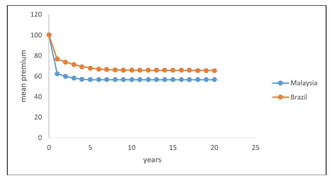
Figure 12.4: Evolution of premium (Malaysia and Brazil)
12.4.5 Convergence Rate
Sometimes we are interested to know the variation between the probability in the n-th year, \(p_{ij}^{(n)}\), and the stationary probability, \(\pi _j\). The variation between the probabilities can be measured using:
\[\left| {average(p_{ij}^{(n)}) - {\pi _j}} \right|\].
Therefore, the total variation can be measured by the sum of variation in all classes:
\[\sum\limits_j {\left| {average(p_{ij}^{(n)}) - {\pi _j}} \right|}\].
The total variation is also called the convergence rate because it measures the convergence rate after \(n\) years (or \(n\) transitions).
Example 8
Provide the total variations (convergence rate) in 20 years under the NCD system in Malaysia, assuming that the probability of claims is Poisson distributed with parameter \(\lambda = 0.10\).
Solution
Using R program, the stationary probabilities are:
\[ \left[ {\begin{array}{*{20}{c}} {{\pi _0}}\\\\{{\pi_1}}\\\\{{\pi _2}}\\\\ {{\pi _3}}\\\\{{\pi _4}}\\\\{{\pi_5}} \end{array}} \right] = \left[ {\begin{array}{*{20}{c}} {0.0952}\\\\{0.0861}\\\\{0.0779}\\\\ {0.0705}\\\\{0.0638}\\\\{0.6064} \end{array}} \right] \]
The transition matrix in the first year is:
\[ {\bf{P}}^{(1)} = \left[ {\begin{array}{*{20}{c}} {0.0952}&{0.9048}&0&0&0&0\\\\ {0.0952}&0&{0.9048}&0&0&0\\\\ {0.0952}&0&0&{0.9048}&0&0\\\\ {0.0952}&0&0&0&{0.9048}&0\\\\ {0.0952}&0&0&0&0&{0.9048}\\\\ {0.0952}&0&0&0&0&{0.9048} \end{array}} \right] \]
The variation can be computed as:
\[ \begin{array}{l} \left| {\sum\limits_i {\frac{p_{i0}^{}}{6}} - {\pi _0}} \right| = 0\\\\ \left|{\sum\limits_i {\frac{p_{i1}^{}}{6}} - {\pi _1}} \right| = 0.0647\\\\ \vdots \\\\ \left| {\sum\limits_i \frac{p_{i5}}{6} - {\pi _5}} \right| = .3048 \end{array} \]
Therefore, the total variation in the first year is \(\sum\limits_j {\left| {\sum\limits_i {\frac{p_{ij}}{6} - {\pi _j}} } \right|} = 0.6096\).
Using R program, the total variations (or convergence rate) in 20 years are:
0.6096, 0.3941, 0.2252, 0.0958, 0, 0, 0, 0, 0, 0, 0, 0, 0, 0, 0, 0, 0, 0, 0, 0.
12.4.6 R Program for Convergence Rate
The following R program can be used to calculate the total variation in the \(n\)th year, and the total variations (convergence rates) in 20 years under the NCD system in Malaysia (the solution in Example 8).
##        [,1]   [,2]   [,3]   [,4]   [,5]   [,6]
## [1,] 0.0952 0.9048 0.0000 0.0000 0.0000 0.0000
## [2,] 0.0952 0.0000 0.9048 0.0000 0.0000 0.0000
## [3,] 0.0952 0.0000 0.0000 0.9048 0.0000 0.0000
## [4,] 0.0952 0.0000 0.0000 0.0000 0.9048 0.0000
## [5,] 0.0952 0.0000 0.0000 0.0000 0.0000 0.9048
## [6,] 0.0952 0.0000 0.0000 0.0000 0.0000 0.9048## [1] 0.09520000+0i 0.08613696+0i 0.07793672+0i 0.07051715+0i 0.06380391+0i
## [6] 0.60640526+0i#create function for total variation in nth year
TV=function(n)
{dif=numeric(0)
for (j in 1:length(SP))
dif[j]=abs(mean(powA(n)[,j])-SP[j])
+ sum(dif)}
#example for n=1
TV(1)## [1] 0.6096105#provide total variations (convergence rate) in 20 years
tot.var=numeric(0)
for (n in 1:20)
tot.var[n]=TV(n)
round(tot.var,4)## [1] 0.6096 0.3941 0.2252 0.0958 0.0000 0.0000 0.0000 0.0000 0.0000 0.0000
## [11] 0.0000 0.0000 0.0000 0.0000 0.0000 0.0000 0.0000 0.0000 0.0000 0.0000Example 9
Provide the total variations (or convergence rate) in 20 years under the NCD system in Brazil, assuming that the number of successive years of claims is distributed as Poisson with parameter \(\lambda = 0.10\)
Solution
Using R program, the total variations (or convergence rates) in 20 years for the NCD system in Brazil are:
1.2617, 1.0536, 0.8465, 0.6412, 0.4362, 0.2316, 0.1531, 0.0747, 0.0480, 0.0232,
0.0145, 0.0071, 0.0043, 0.0021, 0.0013, 0.0006, 0.0004, 0.0002, 0.0001, 0.0001.
Examples 8-9 provide the degree of convergence for two different BMS (two different countries). The Malaysian BMS reaches full stationary only after four years, while the BMS in Brazil takes a longer period. As mentioned in Lemaire (1998), a more sophisticated BMS would converge more slowly, and is considered as a drawback as it takes a longer period to stabilize. The main objective of a BMS is to separate the good drivers from the bad drivers, and thus, it is desirable to have a classification process that can be finalized (or stabilized) as soon as possible.
12.5 BMS and Premium Rating
12.5.2 Frequency Model – Poisson and Negative Binomial Regressions
Let \({({Y_1},{Y_2},...,{Y_n})^T}\) be the vector of count random variables and \(n\) be the sample size. The probability mass function (p.m.f.) for Poisson regression model is,
\[\Pr ({Y_i} = {y_i}) \begin{array}{*{20}{c}} = \frac{{{\exp(- {\mu _i})}{\mu _i}^{y_i}}}{y_i{!}}&{y_i = 0,1,...} \end{array} \]
with mean and variance \(E({Y_i}) = Var({Y_i}) = {\mu _i}\). To take into account non-negative values, the mean, or the fitted value, is assumed to follow a log link, \(E({Y_i}) = {\mu _i} = \exp ({\bf x}_{\bf i}{\bf '\beta })\), where \({\bf{x}}_{\bf i}\) denotes the vector of explanatory variables and \({\bf \beta}\) is the vector of regression parameters. The maximum likelihood estimates can be obtained by maximizing the log likelihood.
The p.m.f. for negative binomial regression model is,
\[ \Pr ({Y_i} = {y_i}) = \frac{{\Gamma ({y_i} + v)}}{y_i{!}\Gamma (v)} \left( \frac{v}{v + {\mu _i}} \right)^v \left( \frac{\mu _i}{v + {\mu _i}} \right)^{y_i},{y_i} = 0,1,2,..., \]
where the mean is \(E({Y_i}) = {\mu _i}\), the variance is \(Var({Y_i}) = {\mu _i}(1 + {v^{ - 1}}{\mu _i}) = {\mu _i}(1 + a{\mu _i})\), and \({v^{ - 1}} = a\) denotes the dispersion parameter. The NB regression model reduce to the Poisson regression model in the limit as \(a \to 0\), and display overdispersion when \(a > 0\). The mean can also be assumed to follow the log link, \(E({Y_i}) = {\mu _i} = \exp ({{\bf x}_{\bf i}{\bf{'\beta }}})\), and the maximum likelihood estimates can be obtained by maximizing the log likelihood.