Chapter 14 Dependence Modeling
Chapter Preview. In practice, there are many types of variables that one encounter and the first step in dependence modeling is identifying the type of variable you are dealing with to help direct you to the appropriate technique. This chapter introduces readers to variable types and techniques for modeling dependence or association of multivariate distributions. Section 14.1 provides an overview of the types of variables. Section 14.2 then elaborates basic measures for modeling the dependence between variables.
Section 14.3 introduces a novel approach to modeling dependence using Copulas which is reinforced with practical illustrations in Section 14.4. The types of Copula families and basic properties of Copula functions is explained Section 14.5. The chapter concludes by explaining why the study of dependence modeling is important in Section 14.6.
14.1 Variable Types
In this section, you learn how to:
- Classify variables as qualitative or quantitative.
- Describe multivariate variables.
People, firms, and other entities that we want to understand are described in a dataset by numerical characteristics. As these characteristics vary by entity, they are commonly known as variables. To manage insurance systems, it will be critical to understand the distribution of each variable and how they are associated with one another. It is common for data sets to have many variables (high dimensional) and so it useful to begin by classifying them into different types. As will be seen, these classifications are not strict; there is overlap among the groups. Nonetheless, the grouping summarized in Table 14.1 and explained in the remainder of this section provides a solid first step in framing a data set.
\[ {\small \begin{matrix} \begin{array}{l|l} \hline \textbf{Variable Type} & \textbf{Example} \\\hline Qualitative & \\ \text{Binary} & \text{Sex} \\ \text{Categorical (Unordered, Nominal)} & \text{Territory (e.g., state/province) in which an insured resides} \\ \text{Ordered Category (Ordinal)} & \text{Claimant satisfaction (five point scale ranging from 1=dissatisfied} \\ & ~~~ \text{to 5 =satisfied)} \\\hline Quantitative & \\ \text{Continuous} & \text{Policyholder's age, weight, income} \\ \text{Discrete} & \text{Amount of deductible (0, 250, 500, and 1000)} \\ \text{Count} & \text{Number of insurance claims} \\ \text{Combinations of} & \text{Policy losses, mixture of 0's (for no loss)} \\ ~~~ \text{Discrete and Continuous} & ~~~\text{and positive claim amount} \\ \text{Interval Variable} & \text{Driver Age: 16-24 (young), 25-54 (intermediate),} \\ & ~~~\text{55 and over (senior)} \\ \text{Circular Data} & \text{Time of day measures of customer arrival} \\ \hline Multivariate ~ Variable & \\ \text{High Dimensional Data} & \text{Characteristics of a firm purchasing worker's compensation} \\ & ~~~\text{insurance (location of plants, industry, number of employees,} \\ &~~~\text{and so on)} \\ \text{Spatial Data} & \text{Longitude/latitude of the location an insurance hailstorm claim} \\ \text{Missing Data} & \text{Policyholder's age (continuous/interval) and "-99" for} \\ &~~~ \text{"not reported," that is, missing} \\ \text{Censored and Truncated Data} & \text{Amount of insurance claims in excess of a deductible} \\ \text{Aggregate Claims} & \text{Losses recorded for each claim in a motor vehicle policy.} \\ \text{Stochastic Process Realizations} & \text{The time and amount of each occurrence of an insured loss} \\ \hline \end{array} \end{matrix}} \]
Table 14.1 : Variable types
In data analysis, it is important to understand what type of variable you are working with. For example, Consider a pair of random variables (Coverage,Claim) from the LGPIF data introduced in chapter 1 as displayed in Figure 14.1 below. We would like to know whether the distribution of Coverage depends on the distribution of Claim or whether they are statistically independent. We would also want to know how the Claim distribution depends on the EntityType variable. Because the EntityType variable belongs to a different class of variables, modeling the dependence between Claim and Coverage may require a different technique from that of Claim and EntityType.
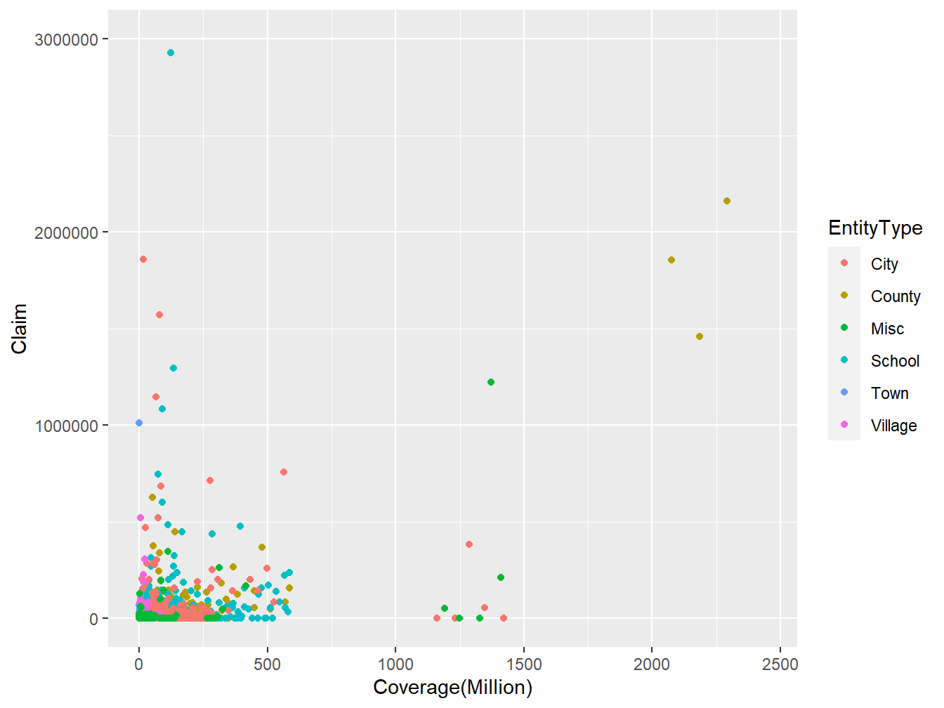
Figure 14.1: Scatter plot of (Coverage,Claim) from LGPIF data
14.1.1 Qualitative Variables
In this sub-section, you learn how to:
- Classify qualitative variables as nominal or ordinal
- Describe binary variable
A qualitative, or categorical variable is one for which the measurement denotes membership in a set of groups, or categories. For example, if you were coding which area of the country an insured resides, you might use a 1 for the northern part, 2 for southern, and 3 for everything else. This location variable is an example of a nominal variable, one for which the levels have no natural ordering. Any analysis of nominal variables should not depend on the labeling of the categories. For example, instead of using a 1,2,3 for north, south, other, I should arrive at the same set of summary statistics if I used a 2,1,3 coding instead, interchanging north and south.
In contrast, an ordinal variable is a type of categorical variable for which an ordering does exist. For example, with a survey to see how satisfied customers are with our claims servicing department, we might use a five point scale that ranges from 1 meaning dissatisfied to a 5 meaning satisfied. Ordinal variables provide a clear ordering of levels of a variable but the amount of separation between levels is unknown.
A binary variable is a special type of categorical variable where there are only two categories commonly taken to be a 0 and a 1. For example, we might code a variable in a dataset to be a 1 if an insured is female and a 0 if male.
14.1.2 Quantitative Variables
In this sub-section, you learn how to:
- Differentiate between continuous and discrete variable
- Use a combination of continuous and discrete variable
- Describe circular data
Unlike a qualitative variable, a quantitative variable is one in which numerical level is a realization from some scale so that the distance between any two levels of the scale takes on meaning. A continuous variable is one that can take on any value within a finite interval. For example, it is common to represent a policyholder’s age, weight, or income, as a continuous variable. In contrast, a discrete variable is one that takes on only a finite number of values in any finite interval. For example, when examining a policyholder’s choice of deductibles, it may be that values of 0, 250, 500, and 1000 are the only possible outcomes. Like an ordinal variable, these represent distinct categories that are ordered. Unlike an ordinal variable, the numerical difference between levels takes on economic meaning. A special type of discrete variable is a count variable, one with values on the nonnegative integers. For example, we will be particularly interested in the number of claims arising from a policy during a given period.
Some variables are inherently a combination of discrete and continuous components. For example, when we analyze the insured loss of a policyholder, we will encounter a discrete outcome at zero, representing no insured loss, and a continuous amount for positive outcomes, representing the amount of the insured loss. Another interesting variation is an interval variable,one that gives a range of possible outcomes.
Circular data represent an interesting category typically not analyzed by insurers. As an example of circular data, suppose that you monitor calls to your customer service center and would like to know when is the peak time of the day for calls to arrive. In this context, one can think about the time of the day as a variable with realizations on a circle, e.g., imagine an analog picture of a clock. For circular data, the distance between observations at 00:15 and 00:45 are just as close as observations 23:45 and 00:15 (here, we use the convention HH:MM means hours and minutes).
14.1.3 Multivariate Variables
In this sub-section, you learn how to:
- Differentiate between univariate and multivariate data
- Handle missing variables
Insurance data typically are multivariate in the sense that we can take many measurements on a single entity. For example, when studying losses associated with a firm’s worker’s compensation plan, we might want to know the location of its manufacturing plants, the industry in which it operates, the number of employees, and so forth. The usual strategy for analyzing multivariate data is to begin by examining each variable in isolation of the others. This is known as a univariate approach.
In contrast, for some variables, it makes little sense to only look at one dimensional aspects. For example, insurers typically organize spatial data by longitude and latitude to analyze the location of weather related insurance claims due hailstorms. Having only a single number, either longitude or latitude, provides little information in understanding geographical location.
Another special case of a multivariate variable, less obvious, involves coding for missing data. Historically, some statistical packages used a -99 to report when a variable, such as policyholder’s age, was not available or not reported. This led to many unsuspecting analysts providing strange statistics when summarizing a set of data. When data are missing, it is better to think about the variable as two dimensions, one to indicate whether or not the variable is reported and the second providing the age (if reported). In the same way, insurance data are commonly censored and truncated. We refer you to Chapter 4 for more on censored and truncated data. Aggregate claims can also be coded as another special type of multivariate variable. We refer you to Chapter 5 for more Aggregate claims.
Perhaps the most complicated type of multivariate variable is a realization of a stochastic process. You will recall that a stochastic process is little more than a collection of random variables. For example, in insurance, we might think about the times that claims arrive to an insurance company in a one year time horizon. This is a high dimensional variable that theoretically is infinite dimensional. Special techniques are required to understand realizations of stochastic processes that will not be addressed here.
14.2 Classic Measures of Scalar Associations
In this section, you learn how to:
- Estimate correlation using Pearson method
- Use rank based measures like Spearman, Kendall to estimate correlation
- Measure dependence using odds ratio, Pearson chi-square and likelihood ratio test statistic
- Use normal-based correlations to quantify associations involving ordinal variables
14.2.1 Association Measures for Quantitative Variables
For this section, consider a pair of random variables \((X,Y)\) having joint distribution function \(F(\cdot)\) and a random sample \((X_i,Y_i), i=1, \ldots, n\). For the continuous case, suppose that \(F(\cdot)\) is absolutely continuous with absolutely continuous marginals.
14.2.1.1 Pearson Correlation
Define the sample covariance function \(\widehat{Cov}(X,Y) = \frac{1}{n} \sum_{i=1}^n (X_i - \bar{X})(Y_i - \bar{Y})\), where \(\bar{X}\) and \(\bar{Y}\) are the sample means of \(X\) and \(Y\), respectively. Then, the product-moment (Pearson) correlation can be written as
\[\begin{equation*} r = \frac{\widehat{Cov}(X,Y)}{\sqrt{\widehat{Cov}(X,X)\widehat{Cov}(Y,Y)}}. \end{equation*}\]
The correlation statistic \(r\) is widely used to capture linear association between random variables. It is a (nonparametric) estimator of the correlation parameter \(\rho\), defined to be the covariance divided by the product of standard deviations. In this sense, it captures association for any pair of random variables.
This statistic has several important features. Unlike regression estimators, it is symmetric between random variables, so the correlation between \(X\) and \(Y\) equals the correlation between \(Y\) and \(X\). It is unchanged by linear transformations of random variables (up to sign changes) so that we can multiply random variables or add constants as is helpful for interpretation. The range of the statistic is \([-1,1]\) which does not depend on the distribution of either \(X\) or \(Y\).
Further, in the case of independence, the correlation coefficient \(r\) is 0. However, it is well known that zero correlation does not imply independence, except for normally distributed random variables. The correlation statistic \(r\) is also a (maximum likelihood) estimator of the association parameter for bivariate normal distribution. So, for normally distributed data, the correlation statistic \(r\) can be used to assess independence. For additional interpretations of this well-known statistic, readers will enjoy (Lee Rodgers and Nicewander 1998).
You can obtain the Pearson correlation statistic \(r\) using the cor() function in R and selecting the pearson method. This is demonstrated below by using the Coverage rating variable in millions of dollars and Claim amount variable in dollars from the LGPIF data introduced in chapter 1.
R Code for Pearson Correlation Statistic
From R output above, \(r=0.31\) , which indicates a positive association between Claim and Coverage. This means that as the coverage amount of a policy increases we expect claim to increase.
14.2.2 Rank Based Measures
14.2.2.1 Spearman’s Rho
The Pearson correlation coefficient does have the drawback that it is not invariant to nonlinear transforms of the data. For example, the correlation between \(X\) and \(\ln Y\) can be quite different from the correlation between \(X\) and \(Y\). As we see from the R code for Pearson correlation statistic above, the correlation statistic \(r\) between Coverage rating variable in logarithmic millions of dollars and Claim amounts variable in dollars is \(0.1\) as compared to \(0.31\) when we calculate the correlation between Coverage rating variable in millions of dollars and Claim amounts variable in dollars. This limitation is one reason for considering alternative statistics.
Alternative measures of correlation are based on ranks of the data. Let \(R(X_j)\) denote the rank of \(X_j\) from the sample \(X_1, \ldots, X_n\) and similarly for \(R(Y_j)\). Let \(R(X) = \left(R(X_1), \ldots, R(X_n)\right)'\) denote the vector of ranks, and similarly for \(R(Y)\). For example, if \(n=3\) and \(X=(24, 13, 109)\), then \(R(X)=(2,1,3)\). A comprehensive introduction of rank statistics can be found in, for example, (Hettmansperger 1984). Also, ranks can be used to obtain the empirical distribution function, refer to section 4.1.1 for more on the empirical distribution function.
With this, the correlation measure of (Spearman 1904) is simply the product-moment correlation computed on the ranks: \[\begin{equation*} r_S = \frac{\widehat{Cov}(R(X),R(Y))}{\sqrt{\widehat{Cov}(R(X),R(X))\widehat{Cov}(R(Y),R(Y))}} = \frac{\widehat{Cov}(R(X),R(Y))}{(n^2-1)/12} . \end{equation*}\]
You can obtain the Spearman correlation statistic \(r_S\) using the cor() function in R and selecting the spearman method. From below, the Spearman correlation between the Coverage rating variable in millions of dollars and Claim amount variable in dollars is \(0.41\).
R Code for Spearman Correlation Statistic
We can show that the Spearman correlation statistic is invariant under strictly increasing transformations. From the R Code for Spearman correlation statistic above, \(r_S=0.41\) between the Coverage rating variable in logarithmic millions of dollars and Claim amount variable in dollars.
14.2.2.2 Kendall’s Tau
An alternative measure that uses ranks is based on the concept of concordance. An observation pair \((X,Y)\) is said to be concordant (discordant) if the observation with a larger value of \(X\) has also the larger (smaller) value of \(Y\). Then \(\Pr(concordance) = \Pr[ (X_1-X_2)(Y_1-Y_2) >0 ]\) , \(\Pr(discordance) = \Pr[ (X_1-X_2)(Y_1-Y_2) <0 ]\), \(\Pr(tie) = \Pr[ (X_1-X_2)(Y_1-Y_2) =0 ]\) and
\[\begin{eqnarray*} \tau(X,Y)= \Pr(concordance) - \Pr(discordance) = 2\Pr(concordance) - 1 + \Pr(tie). \end{eqnarray*}\]
To estimate this, the pairs \((X_i,Y_i)\) and \((X_j,Y_j)\) are said to be concordant if the product \(sgn(X_j-X_i)sgn(Y_j-Y_i)\) equals 1 and discordant if the product equals -1. Here, \(sgn(x)=1,0,-1\) as \(x>0\), \(x=0\), \(x<0\), respectively. With this, we can express the association measure of (Kendall 1938), known as Kendall’s tau, as
\[\begin{equation*} \begin{array}{rl} \tau &= \frac{2}{n(n-1)} \sum_{i<j}sgn(X_j-X_i)sgn(Y_j-Y_i)\\ &= \frac{2}{n(n-1)} \sum_{i<j}sgn(R(X_j)-R(X_i))sgn(R(Y_j)-R(Y_i)) \end{array}. \end{equation*}\]
Interestingly, (Hougaard 2000), page 137, attributes the original discovery of this statistic to (Fechner 1897), noting that Kendall’s discovery was independent and more complete than the original work.
You can obtain the Kendall’s tau, using the cor() function in R and selecting the kendall method. From below, \(\tau=0.32\) between the Coverage rating variable in millions of dollars and Claim amount variable in dollars. When there are ties in the data, the cor() function computes Kendall’s tau_b, as proposed by (Kendall 1945).
R Code for Kendall’s Tau
Also,to show that the Kendall’s tau is invariate under strictly increasing transformations , \(\tau=0.32\) between the Coverage rating variable in logarithmic millions of dollars and Claim amount variable in dollars.
14.2.3 Nominal Variables
14.2.3.1 Bernoulli Variables
To see why dependence measures for continuous variables may not be the best for discrete variables, let us focus on the case of Bernoulli variables that take on simple binary outcomes, 0 and 1. For notation, let \(\pi_{jk} = \Pr(X=j, Y=k)\) for \(j,k=0,1\) and let \(\pi_X=\Pr(X=1)\) and similarly for \(\pi_Y\). Then, the population version of the product-moment (Pearson) correlation can be easily seen to be \[\begin{eqnarray*} \rho = \frac{\pi_{11} - \pi_X \pi_Y}{\sqrt{\pi_X(1-\pi_X)\pi_Y(1-\pi_Y)}} . \end{eqnarray*}\] Unlike the case for continuous data, it is not possible for this measure to achieve the limiting boundaries of the interval \([-1,1]\). To see this, students of probability may recall the Fr\(\acute{e}\)chet-H\(\ddot{o}\)effding bounds for a joint distribution that turn out to be \(\max\{0, \pi_X+\pi_Y-1\} \le \pi_{11} \le \min\{\pi_X,\pi_Y\}\) for this joint probability. This limit on the joint probability imposes an additional restriction on the Pearson correlation. As an illustration, assume equal probabilities \(\pi_X =\pi_Y = \pi > 1/2\). Then, the lower bound is \[\begin{eqnarray*} \frac{2\pi - 1 - \pi^2}{\pi(1-\pi)} = -\frac{1-\pi}{\pi} . \end{eqnarray*}\] For example, if \(\pi=0.8\), then the smallest that the Pearson correlation could be is -0.25. More generally, there are bounds on \(\rho\) that depend on \(\pi_X\) and \(\pi_Y\) that make it difficult to interpret this measure.
As noted by (Bishop, Fienberg, and Holland 1975) (page 382), squaring this correlation coefficient yields the Pearson chi-square statistic (introduced in chapter 2) . Despite the boundary problems described above, this feature makes the Pearson correlation coefficient a good choice for describing dependence with binary data. The other is the odds ratio, described as follows.
As an alternative measure for Bernoulli variables, the odds ratio is given by \[\begin{eqnarray*} OR(\pi_{11}) = \frac{\pi_{11} \pi_{00}}{\pi_{01} \pi_{10}} = \frac{\pi_{11} \left( 1+\pi_{11}-\pi_X -\pi_Y\right)}{(\pi_X-\pi_{11})(\pi_Y- \pi_{11})} . \end{eqnarray*}\] Pleasant calculations show that \(OR(z)\) is \(0\) at the lower Fr\(\acute{e}\)chet-H\(\ddot{o}\)effding bound \(z= \max\{0, \pi_X+\pi_Y-1\}\) and is \(\infty\) at the upper bound \(z=\min\{\pi_X,\pi_Y\}\). Thus, the bounds on this measure do not depend on the marginal probabilities \(\pi_X\) and \(\pi_Y\), making it easier to interpret this measure.
As noted by (Yule 1900), odds ratios are invariant to the labeling of 0 and 1. Further, they are invariant to the marginals in the sense that one can rescale \(\pi_X\) and \(\pi_Y\) by positive constants and the odds ratio remains unchanged. Specifically, suppose that \(a_i\), \(b_j\) are sets of positive constants and that
\[\begin{eqnarray*} \pi_{ij}^{new} &=& a_i b_j \pi_{ij} \end{eqnarray*}\] and \(\sum_{ij} \pi_{ij}^{new}=1.\) Then, \[\begin{eqnarray*} OR^{new} = \frac{(a_1 b_1 \pi_{11})( a_0 b_0 \pi_{00})}{(a_0 b_1 \pi_{01})( a_1 b_0\pi_{10})} = \frac{\pi_{11} \pi_{00}}{\pi_{01} \pi_{10}} =OR^{old} . \end{eqnarray*}\]
For additional help with interpretation, Yule proposed two transforms for the odds ratio, the first in (Yule 1900), \[\begin{eqnarray*} \frac{OR-1}{OR+1}, \end{eqnarray*}\] and the second in (Yule 1912), \[\begin{eqnarray*} \frac{\sqrt{OR}-1}{\sqrt{OR}+1}. \end{eqnarray*}\] Although these statistics provide the same information as is the original odds ration \(OR\), they have the advantage of taking values in the interval \([-1,1]\), making them easier to interpret.
In a later section, we will also see that the marginal distributions have no effect on the Fr\(\acute{e}\)chet-H\(\ddot{o}\)effding of the tetrachoric correlation, another measure of association, see also, (Joe 2014), page 48.
\[ {\small \begin{matrix} \begin{array}{l|rr|r} \hline & \text{Fire5} & & \\ \text{NoClaimCredit} & 0 & 1 & \text{Total} \\ \hline 0 & 1611 & 2175 & 3786 \\ 1 & 897 & 956 & 1853 \\ \hline \text{Total} & 2508 & 3131 & 5639 \\ \hline \end{array} \end{matrix}} \]
Table 14.2 : 2 \(\times\) 2 table of counts for Fire5 and NoClaimCredit variables from LGPIF data.
From Table 14.2, \(OR(\pi_{11})=\frac{1611(956)}{897(2175)}=0.79\). You can obtain the \(OR(\pi_{11})\), using the oddsratio() function from the epitools library in R. From the output below, \(OR(\pi_{11})=0.79\) for the binary variables NoClaimCredit and Fier5 from the LGPIF data.
R Code for Odds Ratios
14.2.3.2 Categorical Variables
More generally, let \((X,Y)\) be a bivariate pair having \(ncat_X\) and \(ncat_Y\) numbers of categories, respectively. For a two-way table of counts, let \(n_{jk}\) be the number in the \(j\)th row, \(k\) column. Let \(n_{j\centerdot}\) be the row margin total, \(n_{\centerdot k}\) be the column margin total and \(n=\sum_{j,k} n_{j,k}\). Define Pearson chi-square statistic as \[\begin{eqnarray*} \chi^2 = \sum_{jk} \frac{(n_{jk}- n_{j\centerdot}n_{\centerdot k}/n)^2}{n_{j\centerdot}n_{\centerdot k}/n} . \end{eqnarray*}\] The likelihood ratio test statistic is \[\begin{eqnarray*} G^2 = 2 \sum_{jk} n_{jk} \ln\frac{n_{jk}}{n_{j\centerdot}n_{\centerdot k}/n} . \end{eqnarray*}\] Under the assumption of independence, both \(\chi^2\) and \(G^2\) have an asymptotic chi-square distribution with \((ncat_X-1)(ncat_Y-1)\) degrees of freedom.
To help see what these statistics are estimating, let \(\pi_{jk} = \Pr(X=j, Y=k)\) and let \(\pi_{X,j}=\Pr(X=j)\) and similarly for \(\pi_{Y,k}\). Assuming that \(n_{jk}/n \approx \pi_{jk}\) for large \(n\) and similarly for the marginal probabilities, we have \[\begin{eqnarray*} \frac{\chi^2}{n} \approx \sum_{jk} \frac{(\pi_{jk}- \pi_{X,j}\pi_{Y,k})^2}{\pi_{X,j}\pi_{Y,k}} \end{eqnarray*}\] and \[\begin{eqnarray*} \frac{G^2}{n} \approx 2 \sum_{jk} \pi_{jk} \ln\frac{\pi_{jk}}{\pi_{X,j}\pi_{Y,k}} . \end{eqnarray*}\] Under the null hypothesis of independence, we have \(\pi_{jk} =\pi_{X,j}\pi_{Y,k}\) and it is clear from these approximations that we anticipate that these statistics will be small under this hypothesis.
Classical approaches, as described in (Bishop, Fienberg, and Holland 1975) (page 374), distinguish between tests of independence and measures of associations. The former are designed to detect whether a relationship exists whereas the latter are meant to assess the type and extent of a relationship. We acknowledge these differing purposes but also less concerned with this distinction for actuarial applications.
\[ {\small \begin{matrix} \begin{array}{l|rr} \hline & \text{NoClaimCredit} & \\ \text{EntityType} & 0 & 1 \\ \hline \text{City} & 644 & 149 \\ \text{County} & 310 & 18 \\ \text{Misc} & 336 & 273 \\ \text{School} & 1103 & 494 \\ \text{Town} & 492 & 479 \\ \text{Village} & 901 & 440 \\ \hline \end{array} \end{matrix}} \]
Table 14.3 : Two-way table of counts for EntityType and NoClaimCredit variables from LGPIF data.
You can obtain the Pearson chi-square statistic, using the chisq.test() function from the MASS library in R. Here, we test whether the EntityType variable is independent of NoClaimCredit variable using Table 14.3.
R Code for Pearson Chi-square Statistic
As the p-value is less than the .05 significance level, we reject the null hypothesis that the EntityType is independent of NoClaimCredit.
Furthermore, you can obtain the likelihood ratio test statistic , using the likelihood.test() function from the Deducer library in R. From below, we test whether the EntityType variable is independent of NoClaimCredit variable from the LGPIF data. Same conclusion is drawn as the Pearson chi-square test.
R Code for Likelihood Ratio Test Statistic
14.2.4 Ordinal Variables
As the analyst moves from the continuous to the nominal scale, there are two main sources of loss of information (Bishop, Fienberg, and Holland 1975) (page 343). The first is breaking the precise continuous measurements into groups. The second is losing the ordering of the groups. So, it is sensible to describe what we can do with variables that in discrete groups but where the ordering is known.
As described in Section 14.1.1, ordinal variables provide a clear ordering of levels of a variable but distances between levels are unknown. Associations have traditionally been quantified parametrically using normal-based correlations and nonparametrically using Spearman correlations with tied ranks.
14.2.4.1 Parametric Approach Using Normal Based Correlations
Refer to page 60, Section 2.12.7 of (Joe 2014). Let \((y_1,y_2)\) be a bivariate pair with discrete values on \(m_1, \ldots, m_2\). For a two-way table of ordinal counts, let \(n_{st}\) be the number in the \(s\)th row, \(t\) column. Let \((n_{m_1\centerdot}, \ldots, n_{m_2\centerdot})\) be the row margin total, \((n_{\centerdot m_1}, \ldots, n_{\centerdot m_2})\) be the column margin total and \(n=\sum_{s,t} n_{s,t}\).
Let \(\hat{\xi}_{1s} = \Phi^{-1}((n_{m_1}+\cdots+n_{s\centerdot})/n)\) for \(s=m_1, \ldots, m_2\) be a cutpoint and similarly for \(\hat{\xi}_{2t}\). The polychoric correlation, based on a two-step estimation procedure, is
\[\begin{eqnarray*} \begin{array}{cr} \hat{\rho_N} &=\text{argmax}_{\rho} \sum_{s=m_1}^{m_2} \sum_{t=m_1}^{m_2} n_{st} \log\left\{ \Phi_2(\hat{\xi}_{1s}, \hat{\xi}_{2t};\rho) -\Phi_2(\hat{\xi}_{1,s-1}, \hat{\xi}_{2t};\rho) \right.\\ & \left. -\Phi_2(\hat{\xi}_{1s}, \hat{\xi}_{2,t-1};\rho) +\Phi_2(\hat{\xi}_{1,s-1}, \hat{\xi}_{2,t-1};\rho) \right\} \end{array} \end{eqnarray*}\]
It is called a tetrachoric correlation for binary variables.
\[ {\small \begin{matrix} \begin{array}{l|rr} \hline & \text{NoClaimCredit} & \\ \text{AlarmCredit} & 0 & 1 \\ \hline 1 & 1669 & 942 \\ 2 & 121 & 118 \\ 3 & 195 & 132 \\ 4 & 1801 & 661 \\ \hline \end{array} \end{matrix}} \]
Table 14.4 : Two-way table of counts for AlarmCredit and NoClaimCredit variables from LGPIF data.
You can obtain the polychoric or tetrachoric correlation using the polychoric() or tetrachoric() function from the psych library in R. The polychoric correlation is illustrated using Table 14.4. \(\hat{\rho}_N=-0.14\), which means that there is a negative relationship between AlarmCredit and NoClaimCredit.
R Code for Polychoric Correlation
14.2.5 Interval Variables
As described in Section 14.1.2, interval variables provide a clear ordering of levels of a variable and the numerical distance between any two levels of the scale can be readily interpretable. For example, drivers age group variable is an interval variable.
For measuring association, both the continuous variable and ordinal variable approaches make sense. The former takes advantage of knowledge of the ordering although assumes continuity. The latter does not rely on the continuity but also does not make use of the information given by the distance between scales.
14.2.6 Discrete and Continuous Variables
The polyserial correlation is defined similarly, when one variable (\(y_1\)) is continuous and the other (\(y_2\)) ordinal. Define \(z\) to be the normal score of \(y_1\). The polyserial correlation is
\[\begin{eqnarray*} \hat{\rho_N} = \text{argmax}_{\rho} \sum_{i=1}^n \log\left\{ \phi(z_{i1})\left[ \Phi(\frac{\hat{\xi}_{2,y_{i2}} - \rho z_{i1}} {(1-\rho^2)^{1/2}}) -\Phi(\frac{\hat{\xi}_{2,y_{i2-1}} - \rho z_{i1}} {(1-\rho^2)^{1/2}}) \right] \right\} \end{eqnarray*}\]
The biserial correlation is defined similarly, when one variable is continuous and the other binary.
\[ {\small \begin{matrix} \begin{array}{l|r|r} \hline \text{NoClaimCredit} & \text{Mean} &\text{Total} \\ & \text{Claim} &\text{Claim} \\ \hline 0 & 22,505 & 85,200,483 \\ 1 & 6,629 & 12,282,618 \\ \hline \end{array} \end{matrix}} \]
Table 14.5 : Summary of Claim by NoClaimCredit variable from LGPIF data.
You can obtain the polyserial or biserial correlation using the polyserial() or biserial() function from the psych library in R. Table 14.5 gives the summary of Claim by NoClaimCredit and the biserial correlation is illustrated using R code below. The \(\hat{\rho}_N=-0.04\) which means that there is a negative correlation between Claim and NoClaimCredit.
R Code for Biserial Correlation
14.3 Introduction to Copulas
Copula functions are widely used in statistics and actuarial science literature for dependency modeling.
In this section, you learn how to:
- Describe a multivariate distribution function in terms of a copula function.
A copula is a multivariate distribution function with uniform marginals. Specifically, let \(U_1, \ldots, U_p\) be \(p\) uniform random variables on \((0,1)\). Their distribution function \[{C}(u_1, \ldots, u_p) = \Pr(U_1 \leq u_1, \ldots, U_p \leq u_p),\]
is a copula. We seek to use copulas in applications that are based on more than just uniformly distributed data. Thus, consider arbitrary marginal distribution functions \({F}_1(y_1)\),…,\({F}_p(y_p)\). Then, we can define a multivariate distribution function using the copula such that \[{F}(y_1, \ldots, y_p)= {C}({F}_1(y_1), \ldots, {F}_p(y_p)).\]
Here, \(F\) is a multivariate distribution function in this equation. Sklar (1959) showed that \(any\) multivariate distribution function \(F\), can be written in the form of this equation, that is, using a copula representation.
Sklar also showed that, if the marginal distributions are continuous, then there is a unique copula representation. In this chapter we focus on copula modeling with continuous variables. For discrete case, readers can see (Joe 2014) and (Genest and Nešlohva 2007).
For bivariate case, \(p=2\) , the distribution function of two random variables can be written by the bivariate copula function: \[{C}(u_1, \, u_2) = \Pr(U_1 \leq u_1, \, U_2 \leq u_2),\]
\[{F}(y_1, \, y_2)= {C}({F}_1(y_1), \, {F}_p(y_2)).\]
To give an example for bivariate copula, we can look at Frank’s (1979) copula. The equation is
\[{C}(u_1,u_2) = \frac{1}{\theta} \ln \left( 1+ \frac{ (\exp(\theta u_1) -1)(\exp(\theta u_2) -1)} {\exp(\theta) -1} \right).\]
This is a bivariate distribution function with its domain on the unit square \([0,1]^2.\) Here \(\theta\) is dependence parameter and the range of dependence is controlled by the parameter \(\theta\). Positive association increases as \(\theta\) increases and this positive association can be summarized with Spearman’s rho (\(\rho\)) and Kendall’s tau (\(\tau\)). Frank’s copula is one of the commonly used copula functions in the copula literature. We will see other copula functions in Section 14.5.
14.4 Application Using Copulas
In this section, you learn how to:
- Discover dependence structure between random variables
- Model the dependence with a copula function
This section analyzes the insurance losses and expenses data with the statistical programming R. This data set was introduced in (Frees and Valdez 1998) and is now readily available in the copula package. The model fitting process is started by marginal modeling of two variables (\(loss\) and \(expense\)). Then we model the joint distribution of these marginal outcomes.
14.4.1 Data Description
We start with getting a sample (\(n = 1500\)) from the whole data. We consider first two variables of the data; losses and expenses.
- losses : general liability claims from Insurance Services Office, Inc. (ISO)
- expenses : ALAE, specifically attributable to the settlement of individual claims (e.g. lawyer’s fees, claims investigation expenses)
To visualize the relationship between losses and expenses (ALAE), scatterplots in figure ?? are created on the real dollar scale and on the log scale.
R Code for Scatterplots
14.4.2 Marginal Models
We first examine the marginal distributions of losses and expenses before going through the joint modeling. The histograms show that both losses and expenses are right-skewed and fat-tailed.
For marginal distributions of losses and expenses, we consider a Pareto-type distribution, namely a Pareto type II with distribution function
\[ F(y)=1- \left( 1 + \frac{y}{\theta} \right) ^{-\alpha},\] where \(\theta\) is the scale parameter and \(\alpha\) is the shape parameter.
The marginal distributions of losses and expenses are fitted with maximum likelihood. Specifically, we use the \(vglm\) function from the R VGAM package. Firstly, we fit the marginal distribution of expenses .
R Code for Pareto Fitting
We repeat this procedure to fit the marginal distribution of the loss variable. Because the loss data also seems right-skewed and heavy-tail data, we also model the marginal distribution with Pareto II distribution.
R Code for Pareto Fitting
To visualize the fitted distribution of expenses and loss variables, we use the estimated parameters and plot the corresponding distribution function and density function. For more details on marginal model selection, see Chapter 4.
14.4.3 Probability Integral Transformation
The probability integral transformation shows that any continuous variable can be mapped to a \(U(0,1)\) random variable via its distribution function.
Given the fitted Pareto II distribution, the variable expenses is transformed to the variable \(u_1\), which follows a uniform distribution on \([0,1]\):
\[u_1 = 1 - \left( 1 + \frac{ALAE}{\hat{\theta}} \right)^{-\hat{\alpha}}.\]
After applying the probability integral transformation to expenses variable, we plot the histogram of Transformed Alae in Figure 14.2.
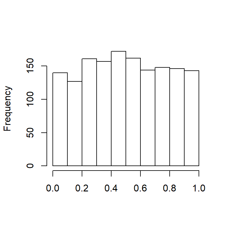
Figure 14.2: Histogram of Transformed Alae
After fitting process,the variable loss is also transformed to the variable \(u_2\), which follows a uniform distribution on \([0,1]\). We plot the histogram of Transformed Loss . As an alternative, the variable loss is transformed to \(normal\) \(scores\) with the quantile function of standard normal distribution. As we see in Figure 14.3, normal scores of the variable loss are approximately marginally standard normal.
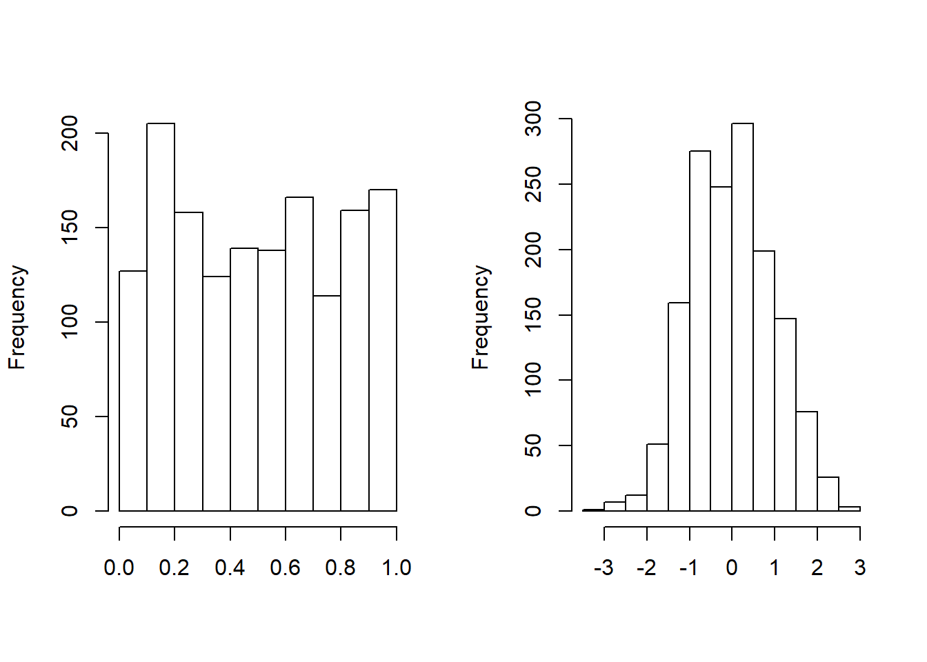
Figure 14.3: Histogram of Transformed Loss. The left-hand panel shows the distribution of probability integral transformed losses. The right-hand panel shows the distribution for the corresponding normal scores.
R Code for Histograms of Transformed Variables
14.4.4 Joint Modeling with Copula Function
Before jointly modeling losses and expenses, we draw the scatterplot of transformed variables \((u_1, u_2)\) and the scatterplot of normal scores in Figure 14.4.
Then we calculate the Spearman’s rho between these two uniform random variables.
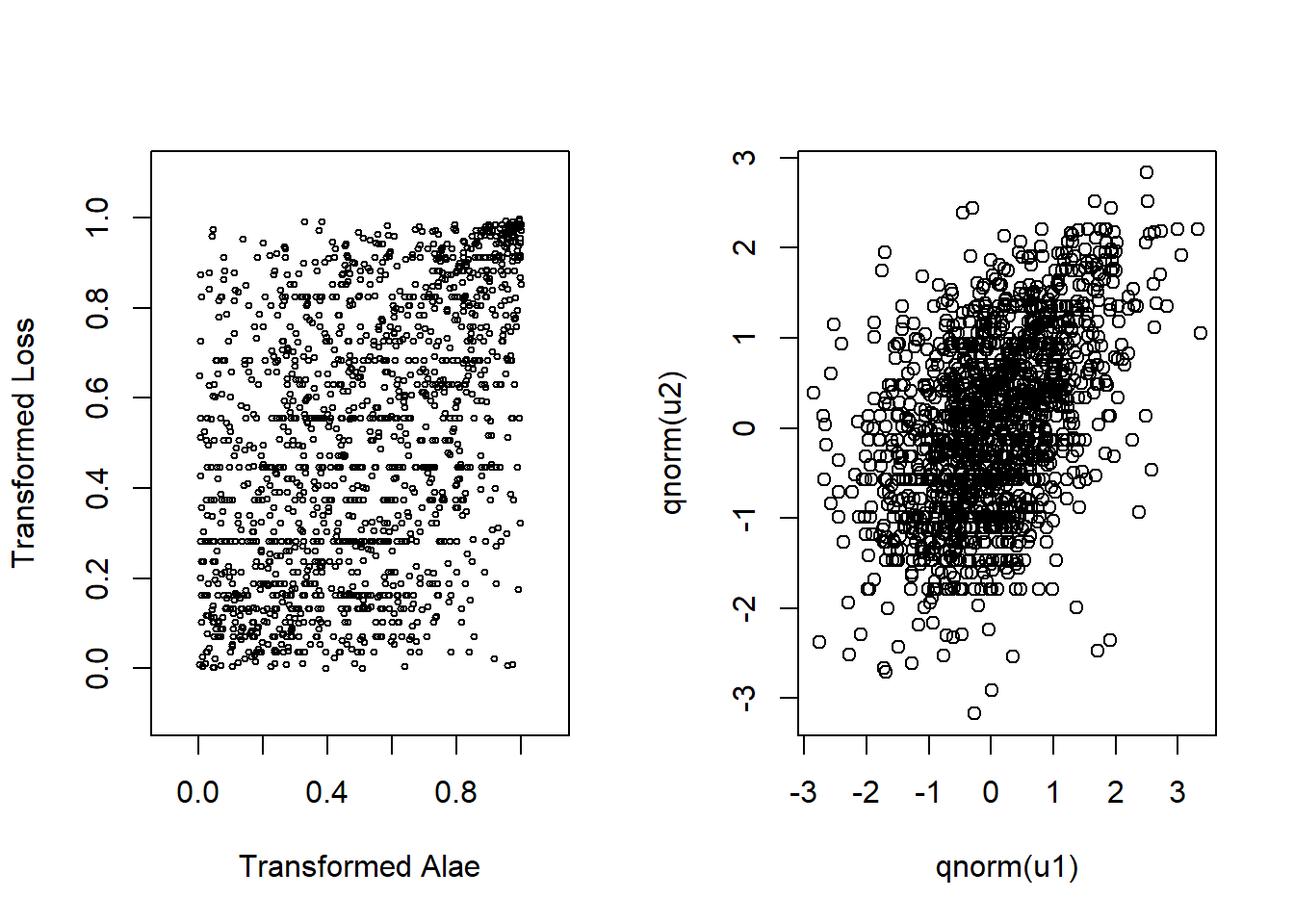
Figure 14.4: Left: Scatter plot for transformed variables. Right:Scatter plot for normal scores
R Code for Scatter Plots and Correlation
Scatter plots and Spearman’s rho correlation value (0.451) shows us there is a positive dependency between these two uniform random variables. It is more clear to see the relationship with normal scores in the second graph. To learn more details about normal scores and their applications in copula modeling, see (Joe 2014).
\((U_1, U_2)\), (\(U_1 = F_1(ALAE)\) and \(U_2=F_2(LOSS)\)), is fit to Frank’s copula with maximum likelihood method.
R Code for Modeling with Frank Copula
The fitted model implies that losses and expenses are positively dependent and their dependence is significant.
We use the fitted parameter to update the Frank’s copula. The Spearman’s correlation corresponding to the fitted copula parameter(3.114) is calculated with the rho function. In this case, the Spearman’s correlation coefficient is 0.462, which is very close to the sample Spearman’s correlation coefficient; 0.452.
R Code for Spearman’s Correlation Using Frank’s Copula
To visualize the fitted Frank’s copula, the distribution function and density function perspective plots are drawn in Figure 14.5.
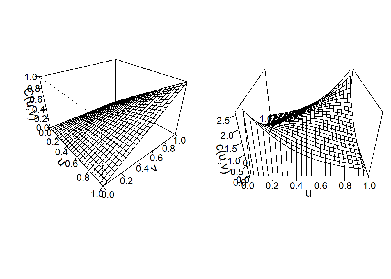
Figure 14.5: Left: Plot for distribution function for Franks Copula. Right:Plot for density function for Franks Copula
R Code for Frank’s Copula Plots
Frank’s copula models positive dependence for this data set, with \(\theta=3.114\). For Frank’s copula, the dependence is related to values of \(\theta\). That is:
- \(\theta=0\): independent copula
- \(\theta>0\): positive dependence
- \(\theta<0\): negative dependence
14.5 Types of Copulas
In this section, you learn how to:
- Define the basic families of the copula functions
- Calculate the association coefficients by the help of copula functions
There are several families of copulas have been described in the literature. Two main families of the copula families are the Archimedian and Elliptical copulas.
14.5.1 Elliptical Copulas
Elliptical copulas are constructed from elliptical distributions. This copula decompose (multivariate) elliptical distributions into their univariate elliptical marginal distributions by Sklar’s theorem (Hofert et al. 2018).
Properties of elliptical copulas are typically obtained from the properties of corresponding elliptical distributions (Hofert et al. 2018).
For example, the normal distribution is a special type of elliptical distribution. To introduce the elliptical class of copulas, we start with the familiar multivariate normal distribution with probability density function \[\phi_N (\mathbf{z})= \frac{1}{(2 \pi)^{p/2}\sqrt{\det \boldsymbol \Sigma}} \exp\left( -\frac{1}{2} \mathbf{z}^{\prime} \boldsymbol \Sigma^{-1}\mathbf{z}\right).\]
Here, \(\boldsymbol \Sigma\) is a correlation matrix, with ones on the diagonal. Let \(\Phi\) and \(\phi\) denote the standard normal distribution and density functions. We define the Gaussian (normal) copula density function as
\[{c}_N(u_1, \ldots, u_p) = \phi_N \left(\Phi^{-1}(u_1), \ldots, \Phi^{-1}(u_p) \right) \prod_{j=1}^p \frac{1}{\phi(\Phi^{-1}(u_j))}.\]
As with other copulas, the domain is the unit cube \([0,1]^p\).
Specifically, a \(p\)-dimensional vector \({z}\) has an \({elliptical}\) \({distribution}\) if the density can be written as \[h_E (\mathbf{z})= \frac{k_p}{\sqrt{\det \boldsymbol \Sigma}} g_p \left( \frac{1}{2} (\mathbf{z}- \boldsymbol \mu)^{\prime} \boldsymbol \Sigma^{-1}(\mathbf{z}- \boldsymbol \mu) \right).\]
We will use elliptical distributions to generate copulas. Because copulas are concerned primarily with relationships, we may restrict our considerations to the case where \(\mu = \mathbf{0}\) and \(\boldsymbol \Sigma\) is a correlation matrix. With these restrictions, the marginal distributions of the multivariate elliptical copula are identical; we use \(H\) to refer to this marginal distribution function and \(h\) is the corresponding density. This marginal density is \(h(z) = k_1 g_1(z^2/2).\)
We are now ready to define the \(elliptical\) \(copula\), a function defined on the unit cube \([0,1]^p\) as
\[{c}_E(u_1, \ldots, u_p) = h_E \left(H^{-1}(u_1), \ldots, H^{-1}(u_p) \right) \prod_{j=1}^p \frac{1}{h(H^{-1}(u_j))}.\]
In the elliptical copula family, the function \(g_p\) is known as a generator in that it can be used to generate alternative distributions.
\[ \small\begin{array}{lc} \hline & Generator \\ Distribution & \mathrm{g}_p(x) \\ \hline \text{Normal distribution} & e^{-x}\\ \text{t-distribution with r degrees of freedom} & (1+2x/r)^{-(p+r)/2}\\ \text{Cauchy} & (1+2x)^{-(p+1)/2}\\ \text{Logistic} & e^{-x}/(1+e^{-x})^2\\ \text{Exponential power} & \exp(-rx^s)\\ \hline \end{array} \]
Table 14.6 : Distribution and Generator Functions (\(\mathrm{g}_p(x)\)) for Selected Elliptical Copulas
Most empirical work focuses on the normal copula and \(t\)-copula. That is, \(t\)-copulas are useful for modeling the dependency in the tails of bivariate distributions, especially in financial risk analysis applications.
The \(t\)-copulas with same association parameter in varying the degrees of freedom parameter show us different tail dependency structures. For more information on about \(t\)-copulas readers can see (Joe 2014), (Hofert et al. 2018).
14.5.2 Archimedian Copulas
This class of copulas are constructed from a \(generator\) function,which is \(\mathrm{g}(\cdot)\) is a convex, decreasing function with domain [0,1] and range \([0, \infty)\) such that \(\mathrm{g}(0)=0\). Use \(\mathrm{g}^{-1}\) for the inverse function of \(\mathrm{g}\). Then the function
\[\mathrm{C}_{\mathrm{g}}(u_1, \ldots, u_p) = \mathrm{g}^{-1} \left(\mathrm{g}(u_1)+ \cdots + \mathrm{g}(u_p) \right)\]
is said to be an Archimedean copula. The function \(\mathrm{g}\) is known as the generator of the copula \(\mathrm{C}_{\mathrm{g}}\).
For bivariate case; \(p=2\) , Archimedean copula function can be written by the function
\[\mathrm{C}_{\mathrm{g}}(u_1, \, u_2) = \mathrm{g}^{-1} \left(\mathrm{g}(u_1) + \mathrm{g}(u_2) \right).\]
Some important special cases of Archimedean copulas are Frank copula, Clayton/Cook-Johnson copula, Gumbel/Hougaard copula. This copula classes are derived from different generator functions.
We can remember that we mentioned about Frank’s copula with details in Section 14.3 and in Section 14.4. Here we will continue to express the equations for Clayton copula and Gumbel/Hougaard copula.
14.5.2.1 Clayton Copula
For \(p=2\), the Clayton copula is parameterized by \(\theta \in [-1,\infty)\) is defined by \[C_{\theta}^C(u)=\max\{u_1^{-\theta}+u_2^{-\theta}-1,0\}^{1/\theta}, \quad u\in[0,1]^2.\]
This is a bivariate distribution function of Clayton copula defined in unit square \([0,1]^2.\) The range of dependence is controlled by the parameter \(\theta\) as the same as Frank copula.
14.5.2.2 Gumbel-Hougaard copula
The Gumbel-Hougaarg copula is parametrized by \(\theta \in [1,\infty)\) and defined by \[C_{\theta}^{GH}(u)=\exp\left(-\left(\sum_{i=1}^2 (-\log u_i)^{\theta}\right)^{1/\theta}\right), \quad u\in[0,1]^2.\]
Readers seeking deeper background on Archimedean copulas can see Joe (2014), Frees and Valdez (1998), and Genest and Mackay (1986).
14.5.3 Properties of Copulas
14.5.3.1 Bounds on Association
Like all multivariate distribution functions, copulas are bounded. The Fr\('{e}\)chet-Hoeffding bounds are
\[\max( u_1 +\cdots+ u_p + p -1, 0) \leq \mathrm{C}(u_1, \ldots, u_p) \leq \min (u_1, \ldots,u_p).\]
To see the right-hand side of the equation, note that \[\mathrm{C}(u_1,\ldots, u_p) = \Pr(U_1 \leq u_1, \ldots, U_p \leq u_p) \leq \Pr(U_j \leq u_j)\], for \(j=1,\ldots,p\). The bound is achieved when \(U_1 = \cdots = U_p\). To see the left-hand side when \(p=2\), consider \(U_2=1-U_1\). In this case, if \(1-u_2 < u_1\) then \(\Pr(U_1 \leq u_1, U_2 \leq u_2) = \Pr ( 1-u_2 \leq U_1 < u_1) =u_1+u_2-1.\) (Nelson 1997)
The product copula is \(\mathrm{C}(u_1,u_2)=u_1u_2\) is the result of assuming independence between random variables.
The lower bound is achieved when the two random variables are perfectly negatively related (\(U_2=1-U_1\)) and the upper bound is achieved when they are perfectly positively related (\(U_2=U_1\)).
We can see The Frechet-Hoeffding bounds for two random variables in the Figure 14.6.
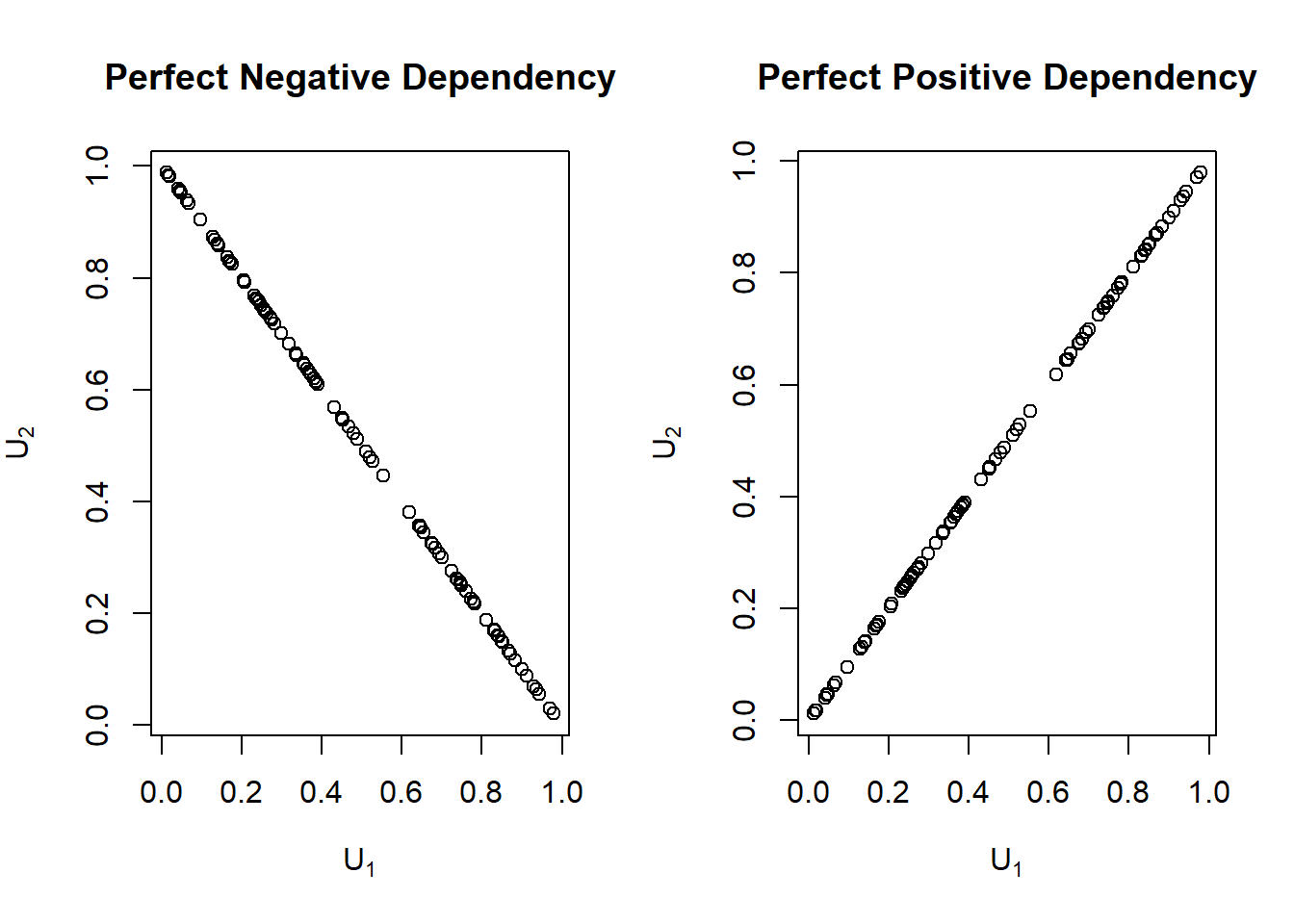
Figure 14.6: Perfect Positive and Perfect negative dependence plots
R Code for Frechet-Hoeffding Bounds for Two Random Variables
14.5.3.2 Measures of Association
Schweizer and Wolff (1981) established that the copula accounts for all the dependence between two random variables, \(Y_1\) and \(Y_2\), in the following sense. Consider m\(_1\) and m\(_2\), strictly increasing functions. Thus, the manner in which \(Y_1\) and \(Y_2\) “move together” is captured by the copula, regardless of the scale in which each variable is measured.
Schweizer and Wolff also showed the two standard nonparametric measures of association could be expressed solely in terms of the copula function. Spearman’s correlation coefficient is given by
\[= 12 \int \int \left\{\mathrm{C}(u,v) - uv \right\} du dv.\]
Kendall’s tau is given by
\[= 4 \int \int \mathrm{C}(u,v)d\mathrm{C}(u,v) - 1 .\]
For these expressions, we assume that \(Y_1\) and \(Y_2\) have a jointly continuous distribution function. Further, the definition of Kendall’s tau uses an independent copy of (\(Y_1\), \(Y_2\)), labeled (\(Y_1^{\ast}\), \(Y_2^{\ast}\)), to define the measure of “concordance.” the widely used Pearson correlation depends on the margins as well as the copula. Because it is affected by non-linear changes of scale.
14.5.3.3 Tail Dependency
There are some applications in which it is useful to distinguish by the part of the distribution in which the association is strongest. For example, in insurance it is helpful to understand association among the largest losses, that is, association in the right tails of the data.
To capture this type of dependency, we use the right-tail concentration function. The function is
\[R(z) = \frac{\Pr(U_1 >z, U_2 > z)}{1-z} =\Pr(U_1 > z | U_2 > z) =\frac{1 - 2z + \mathrm{C}(z,z)}{1-z} .\]
From this equation , \(R(z)\) will equal to \(z\) under independence. Joe (1997) uses the term “upper tail dependence parameter” for \(R = \lim_{z \rightarrow 1} R(z)\). Similarly, the left-tail concentration function is
\[L(z) = \frac{\Pr(U_1 \leq z, U_2 \leq z)}{z}=\Pr(U_1 \leq z | U_2 \leq z) =\frac{ \mathrm{C}(z,z)}{1-z}.\]
Tail dependency concentration function captures the probability of two random variables both catching up extreme values.
We calculate the left and right tail concentration functions for four different types of copulas; Normal, Frank,Gumbel and t copula. After getting tail concentration functions for each copula, we show concentration function’s values for these four copulas in Table 14.7. As in Venter (2002), we show \(L(z)\) for \(z\leq 0.5\) and \(R(z)\) for \(z>0.5\) in the tail dependence plot in Figure 14.7. We interpret the tail dependence plot, to mean that both the Frank and Normal copula exhibit no tail dependence whereas the \(t\) and the Gumbel may do so. The \(t\) copula is symmetric in its treatment of upper and lower tails.
\[ {\small \begin{matrix} \begin{array}{l|rr} \hline \text{Copula} & \text{Lower} & \text{Upper} \\ \hline \text{Frank} & 0 & 0 \\ \text{Gumbel} & 0 & 0.74 \\ \text{Normal} & 0 & 0 \\ \text{t} & 0.10 & 0.10 \\ \hline \end{array} \end{matrix}} \]
Table 14.7 : Tail concentration function values for different copulas
R Code for Tail Copula Functions for Different Copulas
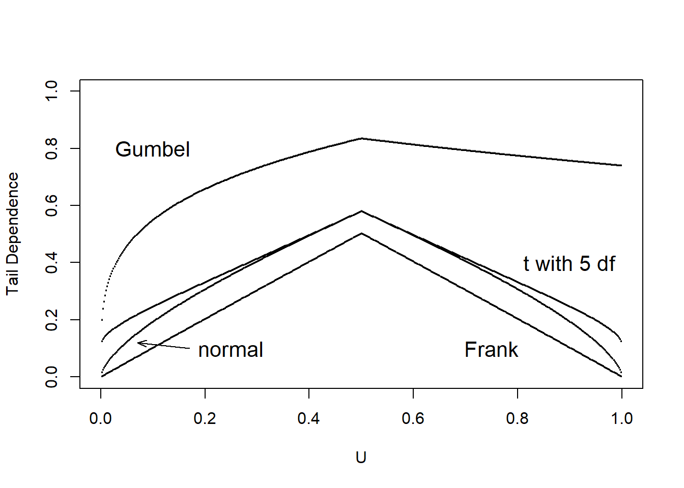
Figure 14.7: Tail dependence plots
R Code for Tail Dependence Plots for Different Copulas
14.6 Why is Dependence Modeling Important?
Dependence Modeling is important because it enables us to understand the dependence structure by defining the relationship between variables in a dataset. In insurance, ignoring dependence modeling may not impact pricing but could lead to misestimation of required capital to cover losses. For instance, from Section 14.4 , it is seen that there was a positive relationship between Loss and Expense. This means that, if there is a large loss then we expect expenses to be large as well and ignoring this relationship could lead to misestimation of reserves.
To illustrate the importance of dependence modeling, we refer you back to Portfolio Management example in Chapter 6 that assumed that the property and liability risks are independent. Here, we incorporate dependence by allowing the 4 lines of business to depend on one another through a Gaussian copula. In Table 14.8, we show that dependence affects the portfolio quantiles (\(VaR_q\)), although not the expect value. For instance , the \(VaR_{0.99}\) for total risk which is the amount of capital required to ensure, with a \(99\%\) degree of certainty that the firm does not become technically insolvent is higher when we incorporate dependence. This leads to less capital being allocated when dependence is ignored and can cause unexpected solvency problems.
\[ {\small \begin{matrix} \begin{array}{l|rrrr} \hline \text{Independent} &\text{Expected} & VaR_{0.9} & VaR_{0.95} & VaR_{0.99} \\ &\text{Value} & & & \\ \hline \text{Retained} & 269 & 300 & 300 & 300 \\ \text{Insurer} & 2,274 & 4,400 & 6,173 & 11,859 \\ \text{Total} & 2,543 & 4,675 & 6,464 & 12,159 \\ \hline \text{Gaussian Copula}&\text{Expected}& VaR_{0.9} & VaR_{0.95} & VaR_{0.99} \\ &\text{Value} & & & \\ \hline \text{Retained} & 269 & 300 & 300 & 300 \\ \text{Insurer} & 2,340 & 4,988 & 7,339 & 14,905 \\ \text{Total} & 2,609 & 5,288 & 7,639 & 15,205 \\ \hline \end{array} \end{matrix}} \]
Table 14.8 : Results for portfolio expected value and quantiles (\(VaR_q\))
R Code for Simulation Using Gaussian Copula
14.7 Further Resources and Contributors
Contributors
- Edward W. (Jed) Frees and Nii-Armah Okine, University of Wisconsin-Madison, and Emine Selin Sarıdaş, Mimar Sinan University, are the principal authors of the initial version of this chapter. Email: jfrees@bus.wisc.edu for chapter comments and suggested improvements.
TS 14.A. Other Classic Measures of Scalar Associations
TS 14.A.1. Blomqvist’s Beta
Blomqvist (1950) developed a measure of dependence now known as Blomqvist’s beta, also called the median concordance coefficient and the medial correlation coefficient. Using distribution functions, this parameter can be expressed as
\[\begin{equation*} \beta = 4F\left(F^{-1}_X(1/2),F^{-1}_Y(1/2) \right) - 1. \end{equation*}\]
That is, first evaluate each marginal at its median (\(F^{-1}_X(1/2)\) and \(F^{-1}_Y(1/2)\), respectively). Then, evaluate the bivariate distribution function at the two medians. After rescaling (multiplying by 4 and subtracting 1), the coefficient turns out to have a range of \([-1,1]\), where 0 occurs under independence.
Like Spearman’s rho and Kendall’s tau, an estimator based on ranks is easy to provide. First write \(\beta = 4C(1/2,1/2)-1 = 2\Pr((U_1-1/2)(U_2-1/2))-1\) where \(U_1, U_2\) are uniform random variables. Then, define \[\begin{equation*} \hat{\beta} = \frac{2}{n} \sum_{i=1}^n I\left( (R(X_{i})-\frac{n+1}{2})(R(Y_{i})-\frac{n+1}{2}) \ge 0 \right)-1 . \end{equation*}\] See, for example, (Joe 2014), page 57 or (Hougaard 2000), page 135, for more details.
Because Blomqvist’s parameter is based on the center of the distribution, it is particularly useful when data are censored; in this case, information in extreme parts of the distribution are not always reliable. How does this affect a choice of association measures? First, recall that association measures are based on a bivariate distribution function. So, if one has knowledge of a good approximation of the distribution function, then calculation of an association measure is straightforward in principle. Second, for censored data, bivariate extensions of the univariate Kaplan-Meier distribution function estimator are available. For example, the version introduced in (Dabrowska 1988) is appealing. However, because of instances when large masses of data appear at the upper range of the data, this and other estimators of the bivariate distribution function are unreliable. This means that, summary measures of the estimated distribution function based on Spearman’s rho or Kendall’s tau can be unreliable. For this situation, Blomqvist’s beta appears to be a better choice as it focuses on the center of the distribution. (Hougaard 2000), Chapter 14, provides additional discussion.
You can obtain the Blomqvist’s beta, using the betan() function from the copula library in R. From below, \(\beta=0.3\) between the Coverage rating variable in millions of dollars and Claim amount variable in dollars.
R Code for Blomqvist’s Beta
In addition,to show that the Blomqvist’s beta is invariate under strictly increasing transformations , \(\beta=0.3\) between the Coverage rating variable in logarithmic millions of dollars and Claim amount variable in dollars.
TS 14.A.2. Nonparametric Approach Using Spearman Correlation with Tied Ranks
For the first variable, the average rank of observations in the \(s\)th row is
\[\begin{equation*} r_{1s} = n_{m_1\centerdot}+ \cdots+ n_{s-1,\centerdot}+ \frac{1}{2} \left(1+ n_{s\centerdot}\right) \end{equation*}\] and similarly \(r_{2t} = \frac{1}{2} \left[(n_{\centerdot m_1}+ \cdots+ n_{\centerdot,s-1}+1)+ (n_{\centerdot m_1}+ \cdots+ n_{\centerdot s})\right]\). With this, we have Spearman’s rho with tied rank is \[\begin{equation*} \hat{\rho}_S = \frac{\sum_{s=m_1}^{m_2} \sum_{t=m_1}^{m_2} n_{st}(r_{1s} - \bar{r})(r_{2t} - \bar{r})} {\left[\sum_{s=m_1}^{m_2}n_{s \centerdot}(r_{1s} - \bar{r})^2 \sum_{t=m_1}^{m_2} n_{\centerdot t}(r_{2t} - \bar{r})^2 \right]^2} \end{equation*}\]
where the average rank is \(\bar{r} = (n+1)/2\).
Click to Show Proof for Special Case: Binary Data.
You can obtain the ties-corrected Spearman correlation statistic \(r_S\) using the cor() function in R and selecting the spearman method. From below \(\hat{\rho}_S=-0.09\).
R Code for Ties-corrected Spearman Correlation
Bibliography
Bishop, Yvonne M., Stephen E. Fienberg, and Paul W. Holland. 1975. Discrete Multivariate Analysis: Theory and Practice. Cambridge [etc.]: MIT.
Blomqvist, Nils. 1950. “On a Measure of Dependence Between Two Random Variables.” The Annals of Mathematical Statistic, 593–600.
Dabrowska, Dorota M. 1988. “Kaplan-Meier Estimate on the Plane.” The Annals of Statistics, 1475–89.
Fechner, G. T. 1897. “Kollektivmasslehre.” Wilhelm Englemann, Leipzig.
Frees, Edward W., and Emiliano A. Valdez. 1998. “Understanding Relationships Using Copulas.” North American Actuarial Journal 2 (01): 1–25.
Genest, Christian, and Josh Mackay. 1986. “The Joy of Copulas: Bivariate Distributions with Uniform Marginals.” The American Statistician 40: 280–83.
Genest, Christian, and Johanna Nešlohva. 2007. “A Primer on Copulas for Count Data.” Journal of the Royal Statistical Society, 475–515.
Hettmansperger, T. P. 1984. Statistical Inference Based on Ranks. Wiley.
Hofert, Marius, Ivan Kojadinovic, Martin Mächler, and Jun Yan. 2018. Elements of Copula Modeling with R. Springer.
Hougaard, P. 2000. Analysis of Multivariate Survival Data. Springer New York.
Joe, Harry. 2014. Dependence Modeling with Copulas. CRC Press.
Kendall, Maurice G. 1938. “A New Measure of Rank Correlation.” Biometrika, 81–93.
Kendall, M. G. 1945. “The Treatment of Ties in Ranking Problems.” Biometrika 33(3): 239–51.
Lee Rodgers, J, and W. A Nicewander. 1998. “Thirteen Ways to Look at the Correlation Coeffeicient.” The American Statistician 42 (01): 59–66.
Nelson, Roger B. 1997. An Introduction to Copulas. Lecture Notes in Statistics 139.
Spearman, C. 1904. “The Proof and Measurement of Association Between Two Things.” The American Journal of Psychology 15 (01): 72–101.
Venter, Gary G. 2002. “Tails of Copulas.” In Proceedings of the Casualty Actuarial Society, 89:68–113. 171.
Yule, G. Udny. 1900. “On the Association of Attributes in Statistics: With Illustrations from the Material of the Childhood Society.” Philosophical Transactions of the Royal Society of London. Series A, Containing Papers of a Mathematical or Physical Character, 257–319.
Yule, G. 1912. “On the Methods of Measuring Association Between Two Attributes.” Journal of the Royal Statistical Society, 579–652.